DESIGN AND OPTIMIZATION A CIRCULAR SHAPE NETWORK ANTENNA MICRO STRIP FOR SOME...
EBDSS Max Research Report - Final
1. 1
IMPLEMENTATION OF A WIDEBAND SPECTRUM SENSING
ALGORITHM USING A SOFTWARE-DEFINED RADIO (SDR)
Max Robertson and Mario Bkassiny
ABSTRACT
This report covers the steps of algorithm creation for wideband spectrum sensing, using raw data
taken from a local software-defined radio. This includes the fundamental idea of Energy Detection Based
Spectrum Sensing and a brief example illustrating this method through simulations obtained via MATLAB.
It will include MATLAB code and functions that are proven to be accurate in reaching this goal. The goal
of this research report is to create an optimized algorithm that successfully senses the local frequency
spectrum, and determines the usage by detecting the un-used portions of the spectrum and relaying this
information back to the user. The aim of this technique is to assess these un-used frequency bands to help
make a more efficient communication system. The simulation of the algorithm was tested first with known
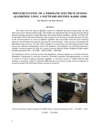
variables, and then tested in the field via a chosen Universal Software Radio Peripheral (USRP) model:
National Instruments (NI) – NI USRP – 2920, 50 MHz – 2200 MHz.
The Introduction will be covered in section I, the Simulations of Known Signals are covered in section II,
Modulation Consideration is covered in section III, Threshold Calculation and Implementation is covered
in section IV, Center Frequency Detection Algorithm is covered in section V, USRP Collected Data
Analysis is covered in section VI, Selected USRP Results are covered in section VII, the Conclusion is
covered in section VIII, and Future Work is covered in section IX.
Universal Software Radio Peripheral (USRP) model: National Instruments (NI) – NI USRP – 2920,
50 MHz – 2200 MHz.
2. 2
I. INTRODUCTION
The idea of Cognitive Radios (CR) is relatively new, much like the age of multimedia
communication, and the manipulation of these CR’s could potentially change the way we communicate
forever. In this report, Energy Detection Based Spectrum Sensing (EDBSS) is the main focus, and as
shown in other studies it proves to be the simplest form of investigation into this problem. Many other
approaches have been proposed, including “Waveform-Based Sensing (WBS), Cyclostaionary-Based
Sensing (CBS), Radio Identification Based Sensing (RIBS),Matched Filtering (MF), and many more; not
to mention the cooperative approach”[1], which simply combines some of the previously stated methods.
The EDBSS approach is the least complex and thus is the least accurate of the methods stated, but in
understanding at this level it can be transferred to the higher levels of complexity. Once the concept of
signal generation has been grasped, digitization and modulation are a key aspect of communication
through CR’s. The MATLAB code used in this report suffices for accurate replication of this experiment.
The parameters of this approach will be stated and justification as to their particular chosen values will be
thorough as well. The results are subject to change if replicated as spectrum usage changes all the time,
the time of day is as variant as the time of year, location too is a large aspect. There are many angles to
cover, and prior knowledge of signal detection would be of great advantage too. The techniques and code
produced in this report is of a university undergraduate level, and therefore has a very basic format. The
first few sections cover an introduction to signal generation and understanding the fundamentals behind
what we are trying to achieve; moving on to more technical code but again explained enough to replicate
with ease. The end goal of this challenge is to see if this idea of spectrum sensing using an autonomous
algorithm will work, first with known data and variables, and then again in the realworld where the
signals are unknown; at least, unknown for now. The first step of this experiment is creating a base line
algorithm, and being able to familiarize oneself with MATLAB and basic signal generation.
II. DETECTION OF SINUSOIDAL SIGNALS USING ENERGY DETECTORS
In this section the report will describe the approach, computation methods and plots obtained from
this EDBSS simulation using MATLAB software. Note that,in this section, the signal generation has
certain parameters; without loss of generality let us assume that the signal is sinusoidal and has a power of
1W. Let us also assume that the carrier frequency is 10MHz. Taking into consideration the Nyquist
property that the sampling rate must be at least twice that of the carrier frequency. To fulfil this
requirement set the sampling rate of the signal to be 100MHz, which is ten times as large as the carrier
frequency. In doing so, the plots produced will be more accurate and have smoother curves, if any. We
also assume that the sensing duration is very small, such that one period ( sT ) is set to 1µs. Remember
that for this simulation we are making the assumption that the signal is sinusoidal and has finite power.
Thus we have:
)cos()( 0tAtx , where 20 t tf0
3. 3
Note that )(tx is considered as a finite-power signal whose power xP can be expressed in function of
the amplitude A.
A very simple proof of this relationship is shown below:
PROOF:
dttx
T
P
To
To
x
2
2
2
0
)(*
1
dttA
T
To
To
2
2
0
22
0
)(cos*
1
dtt
T
A
To
To
2
2
0
0
2
)]2cos(
2
1
2
1[*
)]2sin(
2
1
[*
2
0
00
2 2
2
tt
T
A
To
To
)sin(
2
1
2
)sin(
2
1
22
00
0
0
00
0
0
0
2
T
T
T
T
T
A
2
0
2
2
0
0
2
A
T
T
A
So now we can compute the desired value of A when we have a signal power of 1W. Using the formula
above A= 2 .
MATLAB:
power=1; %signal power (Watts)
fc=10*10^6; %frequency (MHz)
fs=10*fc; %sampling rate > 2*fc (MHz)
T=0:1/fs:1*10^-6; %sensing (micro-sec)
A=sqrt(2); %would solve for A from Power=1W
x=A*sin(2*pi*fc*T); %sinusoidal setup
4. 4
II. A. Spectrum Estimation in the Absence of Noise
The setup is relatively simple, and the parameters can change depending on the user preference or
environment specifications. Now we have a signal with the correct parameters,we need to compute the
Fast-Fourier Transform (FFT) of the function, which ultimately converts the signal from time-domain to
frequency-domain. But the axis in frequency domain are different and require some adjusting when
plotting the signals. We calculate and plot the signal itself in time-domain, then its magnitude spectrum,
then we finish by plotting the associating phase angle spectrum. This is standard procedure for signal
analysis. Note: we must normalize the axis for the FFT plots.
MATLAB:
N=length(x);
n=sqrt(0.1)*randn(1,N);
f0=[-N/2:N/2-1];
f1=f0/N; %This normalizes the frequency from -1/2 to 1/2-1/N
f=f1*fs; %fs is the sampling rate. f is now a vector from -fs/2 to fs/2-fs/N~fs/2
Now we can compute the Fast Fourier Transform of the function x:
MATLAB:
X=fftshift(fft(x)); %fast-fourier transform
X0=abs(X);%Magnitude
X1=angle(X); %angle
6. 6
Magnitude Spectrum of )(tx :
%subplot(312)
%stem(f,X0);
plot(f, X0,'r');
ylabel('|X(f)|');
xlabel('f(Hz)');
title('Magnitude Spectrum |X(f)| in the Absence of Noise');
grid;
figure
-5 -4 -3 -2 -1 0 1 2 3 4 5
x 10
7
0
10
20
30
40
50
60
70
|X(f)|
f(Hz)
Magnitude Spectrum |X(f)| in the Absence of Noise
7. 7
Phase Spectrum of )(tx :
%subplot(313)
%stem(f,X1);
plot(f,X1,'g');
ylabel('<X');
xlabel('f(Hz)');
title('Phase Spectrum in the Absence of Noise');
grid;
figure
These results show how the signal reacts at certain times and frequencies, but it is the first key step in
understanding signal generation and eventually signal manipulation.
-5 -4 -3 -2 -1 0 1 2 3 4 5
x 10
7
-4
-3
-2
-1
0
1
2
3
4
<X
f(Hz)
Phase Spectrum in the Absence of Noise
8. 8
II. B. Spectrum Estimation in the presence of Additive White Gaussian Noise (AWGN)
The setup is essentially the same, except now the signal will have some additional component to show
consideration for Gaussian white noise, which is most likely to occur in real time application, the world is
a busy and noisy place. The easiest approach is to use the same signal generated from before but add a
vector to account for the noise, and for this to be of type Gaussian, we will again assume random Normal
numbers distributed with a mean zero and a certain variance. In this case the variance is the noise power,
so we will assume this to be 0.1 Watts; this parameter can also change depending on scenario or customer
specification. Once we have generated this vector, we can follow the same techniques as previous to
simulate a more realistic setup.
MATLAB:
N=length(x);
n=sqrt(0.1)*randn(1,N);
y=x+n;
Y=fftshift(fft(y)); %y is the time domain signal with N elements
Y0=abs(Y); %The magnitude spectrum with N elements
Y1=angle(Y); %Angle
Note that )()()( tntxty .
10. 10
Magnitude Spectrum of )(ty :
%subplot(312)
%stem(f,Y0);
plot(f, Y0,'r');
ylabel('|Y(f)|');
xlabel('f(Hz)');
title('Magnitude Spectrum |Y(f)| in the presence of AWGN');
grid;
figure
-5 -4 -3 -2 -1 0 1 2 3 4 5
x 10
7
0
10
20
30
40
50
60
70
80
|Y(f)|
f(Hz)
Magnitude Spectrum |Y(f)| in the presence of AWGN
11. 11
Phase Spectrum of )(ty :
%subplot(313)
%stem(f,Y1);
plot(f,Y1,'g');
ylabel('<Y');
xlabel('f(Hz)');
title('Phase Spectrum in the presence of AWGN');
grid;
figure
Notice the changes of these three plots versus the first three plots; this is closer to what you would
expect to see in realworld application of CR’s,there needs to be some sort of accountability for the
inevitable noise. These plots are not as smooth as before due to the stochastic non-deterministic nature of
the noise process.
-5 -4 -3 -2 -1 0 1 2 3 4 5
x 10
7
-4
-3
-2
-1
0
1
2
3
4
<Y
f(Hz)
Phase Spectrum in the presence of AWGN
12. 12
III. DETECTION OF MODULATED SIGNALS
III. A. Generation of Modulated Signals
The signal transmitter is a key component of any communication system. In order to be transmitted
over wireless channels, signals should be modulated according to a certain modulation scheme. The
objective of spectrum sensing is to detect the active wireless signals in a particular RF environment and
identify their characteristics,such as their center frequencies and bandwidths. In this simulation setup, we
assume a certain transmitted digital signal that is modulated as a binary phase shift keying (BPSK). As
shown in the previous section, AWGN can distort the original signal and potentially allow for a large loss
of information. As digital signals are simply ordered sequences of zeros and ones, they can resist this
noise much more efficiently. So, we will use this technique to model a distorted digital signal and propose
a spectrum sensing algorithm to detect wireless signals under AWGN. An explanation of the steps will be
followed with the MATLAB code used to generate and simulate this concept.
Simulation Setup: Firstly, we need a sequence that randomly generates zeros and ones and stores them
in an array of length 100, this number is arbitrary but without loss of generality we will use 100 to
represent the bit generation (100 bits). The bits will be modulated using polar signaling, where we assign
a value of +1V to a value of 0, and -1V to a value of 1. This idea comes from BPSK where these bit
values ([0, 1]) and their corresponding values ( 1 ) can be seen in the complex plane. Also within this
sequence we need a symbol duration, the duration of a single bit: let this equal 1ms (milliseconds). We
also need a sampling period, one that is small would give a better generation and plot of the signal
(smoother curve due to more points), we will let it equal 0.01ms. The main characteristic is using this
Baseband Digital Signal (BDS):
k
ok kTtpbts )(*)( ,
where kb is the randomsequence of { 1 }, k is the bit index, T0 is the bit duration, and )( okTtp is a
shifted rectangular pulse function.
We will use the KRON function in MATLAB to generate this; an array of 100 points for each bit
essentially. Once completed, we will use the same setup as in the previous section with the plot
generation in frequency domain of the Magnitude and Phase Angle, and the use of the FFT once again.
MATLAB:
A_k=randi([0 1],1,100); %random sequence of 0's and 1's (Binary)
B=ones(1,100); %equal in size to A_k to help with Kron function
A_k(A_k > 0.5)= [-1]; %replaces all 1's with -1
A_k(A_k ~= -1)= [1]; %replaces all 0's with 1
B_k = A_k; %new sequence of 1's and -1's
T_o = 1e-3; %bit duration
T_s = 0.01e-3; %sampling period
N=length(s_t);
f0=[-N/2:N/2-1]; %scales the x-axis for frequency domain
13. 13
f1=f0/N; %This normalizes the frequency
f=f1/T_s; %This will be the frequency x-axis (scaled)
Now for generating the plots:
s_t=kron(B_k,B); %s_t is the baseband signal
S_t=fftshift(fft(s_t)); %FFT
Mag_S=abs(S_t); %Magnitude spectrum
Ang_S=angle(S_t); %Phase angle spectrum
)(ts :
%subplot(311)
t=T_s:T_s:100*T_o;
plot(t,s_t,'b')
ylim([-2 2]);
title('The signal S(t)');
xlabel('Bit number in binary sequence {A_k}');
ylabel('Bit value - (HIGH/LOW)');
grid;
figure
0 0.01 0.02 0.03 0.04 0.05 0.06 0.07 0.08 0.09 0.1
-2
-1.5
-1
-0.5
0
0.5
1
1.5
2
The signal S(t)
Bit number in binary sequence Ak
Bitvalue-(HIGH/LOW)
16. 16
Once we have created a Modulated signal we need to create a Digital Modulated Signal (DMS), which
essentially takes the function from previous and multiplying it by a cosine function with a certain carrier
frequency. For the purpose of this signal generation, the top plot is with a carrier frequency of 20 KHz
and the bottom plot is with a carrier frequency of 25 KHz. The same process as before when plotting is
applied here. The important thing to remember here,is that this signal )(ty is what is being transmitted.
MATLAB:
y_t=s_t.*cos(2*pi.*f_c1.*t); %digital modulated signal
Y_t=fftshift(fft(y_t)); %FFT
Mag_Y=abs(Y_t);
Ang_Y=angle(Y_t);
L=length(y_t);
P_s = sum(y_t.^2)/L; %power of modulated signal before transmission
g0=[-L/2:L/2-1];
g1=g0/L;
g=g1/T_s;
:)(tY
%subplot(311)
t=T_s:T_s:100*T_o;
plot(t,y_t,'b') %y_t would vary depending on F_c
ylim([-2 2]);
title('The signal Y(t)-(F_c=20/25KHz)');
xlabel('Bit number in binary sequence {A_k}');
ylabel('Bit value - (HIGH/LOW)');
grid;
figure
17. 17
0 0.01 0.02 0.03 0.04 0.05 0.06 0.07 0.08 0.09 0.1
-2
-1.5
-1
-0.5
0
0.5
1
1.5
2
The signal Y(t)-(Fc
=20KHz)
Bit number in binary sequence Ak
Bitvalue-(HIGH/LOW)
0 0.01 0.02 0.03 0.04 0.05 0.06 0.07 0.08 0.09 0.1
-2
-1.5
-1
-0.5
0
0.5
1
1.5
2
The signal Y(t) -(Fc
=25KHz)
Bit number in binary sequence Ak
Bitvalue-(HIGH/LOW)
20. 20
III. B. Modulated Signal in AWGN Channel
In this section we will cover not only generating a modulated signal but also recognizing the presence
of Gaussian White Noise. The setup and understanding is very similar to that in section II, so far we have
a signal that is being transmitted from one CR to another, and now we have to account or rather add this
noise to our signal. The setup and code is very similar in the fact that we will generate random Gaussian-
distributed numbers with a mean zero and variance equal to the Noise Power. This value is based user
preference,for this example let the noise power ( nP ) equal 0.1Watts. We will take our existing signal:
)(ty from previous, and essentially add some arbitrary Noise Function (NF) such that:
)()()( tntytr , where )(tn is an AWGN signal.
At this point we can note that now we have a signal: )(ty that we have received, and now we essentially
add noise (AWGN): )(tn and now we have some signal )(tr that is essentially our end product. We will
now continue to work with and analyze )(tr .
We can also compute the Signal-to-Noise Ratio (SNR) by taking:
n
s
P
P
10log10 , where sP is the
Signal Power and nP is the Noise Power. For the purpose of this test, by fixing the Signal Power to some
value say 0.5W (Watts) and a false-alarm rate of 0.001; I calculated graphically that the maximum Noise
Power needed would be approximately 10,000W to evaluate a minimum SNR of approximately: -43.0103
MATLAB:
M=length(y_t);
P_n = 0.1; %noise power
n_t = sqrt(P_n)*randn(1,M); %random Gaussian white noise generator
r_t = y_t + n_t; %modulated signal with AWGN signal n(t)
R_t=fftshift(fft(r_t)); %FFT
Mag_R=abs(R_t);
Ang_R=angle(R_t);
h0=[-M/2:M/2-1];
h1=h0/M;
h=h1/T_s;
:)(tr
%subplot(311)
t=T_s:T_s:100*T_o;
plot(t,r_t,'b') %r(t) would vary depending on F_c
ylim([-2 2]);
title('The signal R(t)- (F_c=20/25KHz)');
xlabel('Bit number in binary sequence {A_k}');
ylabel('Bit value - (HIGH/LOW)');
grid;
figure
21. 21
0 0.01 0.02 0.03 0.04 0.05 0.06 0.07 0.08 0.09 0.1
-2
-1.5
-1
-0.5
0
0.5
1
1.5
2
The signal R(t)- (Fc
=20KHz)
Bit number in binary sequence Ak
Bitvalue-(HIGH/LOW)
0 0.01 0.02 0.03 0.04 0.05 0.06 0.07 0.08 0.09 0.1
-2
-1.5
-1
-0.5
0
0.5
1
1.5
2
The signal R(t) - (Fc
=25KHz)
Bit number in binary sequence Ak
Bitvalue-(HIGH/LOW)
24. 24
IV. THRESHOLD DETECTION FOR WIDEBAND SIGNALS
This section is one of the most important, as it will be essentially the point where a signal is declared as
being present or evaluated as being noise. The concept is rather simple, we need to construct some value
η that acts as a threshold for the signal; where graphically if there exists a signal above this value then we
will conclude there exists an Active Frequency (AF) component, any frequency or signal/points below
this threshold line will be evaluated as being interference,a Noise Frequency (NF) component, essentially
no signals present. False-alarm denotes the probability of declaring a signal is present when there is no
active signals. This is equivalent to a Type I error in statistical analysis.
Our proposed detection rule will be based on the Neyman-Pearson (NP) criterion which maximizes the
detection probability, given an upper bound on the false alarm rate. So we will demonstrate how this false
alarm value (alpha) will effect η and ultimately how much/little information is lost. Without loss of
generality (WLOG), we will set alpha equal to 0.1, where alpha is the false alarm probability. We will use
a manipulation of the inverse lower incomplete gamma function to help estimate this threshold value η,
you will see this in the MATLAB code, also note that we are using a SpectralWindow Length (SWL) of
1, as this will make our basic computation easier. We will use this formula [2]:
))(*)1(;(*2 1
LalphaL
,
where
1
is the inverse lower incomplete gamma function
(where:
x
tk
dtetxk
0
1
);( and
0
1
)( dtetk tk
).
In realworld application, the SWL will be larger as it will help increase the detection probability by
smoothing the periodogram of the sensed signal. At this point in the problem we now have a signal that
has been digitally modulated and also has the addition of noise, so the next part is to essentially take the
Periodogram of this function )(tr to estimate the spectraldensity of the signal. Note that this new signal
will have a Chi-Square Distribution with 2P degrees of freedom (d.o.f); )( fR is the Magnitude Spectrum
of )(tr and P is the number of elements in )(tr .The plot is simply [2]:
2
)(*
1
fR
P
MATLAB:
SWL=1; %spectral window length
alpha1=0.1; %False alarm rate
alpha2=0.01;
alpha3=0.001;
P=length(r_t);
pgm=(1/P).*(Mag_R).^2; %periodogram generation
i0=[-P/2:P/2-1];
i1=i0/P;
i=i1/T_s;
25. 25
plot(i,pgm,'m'); %pgm would vary depending on F_c
ylabel('(1/P)*|R(f)|.^2');
xlabel('f(Hz)');
title('Periodogram of r(t) - (F_c=20/25KHz)');
grid;
figure
27. 27
Now if we choose some SWL that is greater than 1, then we create a new smoother graph; this
smoothing process occurs because we plot shifted curves individually then sum them to get an overall
average plot, depending on the SWL essentially implies how many plots will be averaged. We will use
this smoothing expression [2]:
22/)1(
2/)1(
)()(
L
L
nXnT
,
where L=SWL and n=0…,N-1 (N=length of X(n))
The figure above is a graphical representation of the smoothing operation, where SWL=3 for this case.
We will be referencing [3], as in this paper it shows other simulations of how increasing the SWL can
effect SNR.
You can see on the following plots how increasing the SWL can affect the Periodogram; the following
setup will proceed as:
F_c=20KHz plot(SWL=3,7,11)
F_c=25KHz plot(SWL=3,7,11)
MATLAB:
alpha1=0.1; %False alarm rates
alpha2=0.01;
alpha3=0.001;
P1=length(r_t1);
P2=length(r_t2);
pgmn1=(Mag_R1).^2; %This formula comes from the ICC paper
pgmn2=(Mag_R2).^2;
pgm1=(1/P1).*(pgmn1); %This was used previously, won’t be used here
pgm2=(1/P2).*(pgmn2);
i0=[-P1/2:P1/2-1]; %X-axis frequency scaling for periodogram
i1=i0/P1;
i=i1/T_s;
28. 28
SWL1=3; %spectral window length
SWL2=7; %spectral window length
SWL3=11; %spectral window length
Q1=length(r_t1); %X-axis frequency scaling for periodogram
Q2=length(r_t2);
q0=[-Q1/2:Q1/2-1];
q1=q0/Q1;
q=q1/T_s;
%This accounts for all eta values for all SWL’s
eta1_1=2*gammaincinv((1-alpha1),SWL1,'lower'); %threshold value eta1, SWL=3
eta1_2=2*gammaincinv((1-alpha2),SWL1,'lower'); %threshold value eta2, SWL=3
eta1_3=2*gammaincinv((1-alpha3),SWL1,'lower'); %threshold value eta3, SWL=3
eta2_1=2*gammaincinv((1-alpha1),SWL2,'lower'); %threshold value eta1, SWL=7
eta2_2=2*gammaincinv((1-alpha2),SWL2,'lower'); %threshold value eta2, SWL=7
eta2_3=2*gammaincinv((1-alpha3),SWL2,'lower'); %threshold value eta3, SWL=7
eta3_1=2*gammaincinv((1-alpha1),SWL3,'lower'); %threshold value eta1, SWL=11
eta3_2=2*gammaincinv((1-alpha2),SWL3,'lower'); %threshold value eta2, SWL=11
eta3_3=2*gammaincinv((1-alpha3),SWL3,'lower'); %threshold value eta3, SWL=11
This is the main code that produces the new vector T such that it sums the relevant X(n) values depending
on the SWL:
%plots for smoothed periodogram with threshold value
%smoothed periodogram SWL_1_1
SWL1=3; %spectral window length
k1_1=-(SWL1-1)/2; %lower sum
k2_1=(SWL1-1)/2; %upper sum
k3_1=k1_1:k2_1;
T1_1=zeros(1,P1); %creates a vector T for reassignment from for loop
for j_21=1:P1
a1=max(j_21+k1_1,1); %truncation at 1, lower end
b1=min(j_21+k2_1,P1); %truncation at P, upper end
T1_1(j_21)=sum(pgmn1(a1:b1)); %summation over SWL iterations
end
%varying SWL_1_1 %eta and T depend on F_c
plot(i,T1_1,'m',i,eta1_1,'r',i,eta1_2,'b',i,eta1_3,'c');
ylabel('|R(f)|.^2');
xlabel('f(Hz)');
title('Smoothed Periodogram of r(t) - (F_c=20/25KHz) SWL=3 W/eta1,2,3');
grid;
figure
31. 31
As you can see comparing just these three SWL plots that a definitive curve is beginning to appear as the
SWL increases. This same technique, but now applied to 25KHz to show repeatability.
-5 -4 -3 -2 -1 0 1 2 3 4 5
x 10
4
0
0.5
1
1.5
2
2.5
3
3.5
x 10
6
|R(f)|.2
f(Hz)
Smoothed Periodogram of r(t) - (Fc
=20KHz) SWL=11 W/eta1,2,3
34. 34
As you can see comparing just these three SWL plots that a definitive curve is beginning to appear as the
SWL increases for this carrier frequency too.
-5 -4 -3 -2 -1 0 1 2 3 4 5
x 10
4
0
0.5
1
1.5
2
2.5
3
3.5
x 10
6
|R(f)|.2
f(Hz)
Smoothed Periodogram of r(t) - (Fc
=25KHz) SWL=11 W/eta1,2,3
35. 35
This process would be repeated for all threshold values of eta (η) and all SWL values. As you can see
from the plots produced you cannot see the threshold lines clearly, this is why we will use a logarithmic
scale on the y-axis, and the changes will become clearer.
Note: that I have changed the scaling to KHz, essentially the x-axis is divided by 1000,a simple
scaling technique.
MATLAB:
%semilog 1_1
semilogy(i/1000,T1_1,'m');
ylabel('|R(f)|.^2');
xlabel('f(KHz)');
title('Smoothed Periodogram of r(t) - (BSPK signal) - (F_c=20KHz) - Spectral
Window Length=3 - 10,000 samples – SNR=6.9897’);
grid;
hold on
xh1 = [-50 50];
yh1 = [eta1_1 eta1_1];
semilogy(xh1,yh1,'r')
xh2 = [-50 50];
yh2 = [eta1_2 eta1_2];
semilogy(xh2,yh2,'b')
xh3 = [-50 50];
yh3 = [eta1_3 eta1_3];
semilogy(xh3,yh3,'c')
hold off
figure
As you can see from this new scaling technique, the SWL increasing causes the data to shift upwards, we
are essentially obtaining a larger average of plots as the SWL is the dependent variable. The setup of the
following logarithmic plots will be F_c=20KHz (SWL=3,7,11) followed by F_c=25KHz (SWL=3,7,11).
Spectral
Window Length
(SWL)
False-Alarm Probability (alpha) η value
1 0.1 4.6052
1 0.01 9.2103
1 0.001 13.8155
3 0.1 10.6446
3 0.01 16.8119
3 0.001 22.4577
7 0.1 21.0641
7 0.01 29.1412
7 0.001 36.1233
11 0.1 30.8133
11 0.01 40.2894
11 0.001 48.2679
41. 41
As you can see,the plots shift upwards as the SWL increases but also notice how the curve is smoothing-
becoming thinner (Peak to Peak); very similar to the previously described carrier frequency.
NOTE:
A close estimation to the optimal SWL value would be a value above 11 because it is approximately after
this length that the smoothing operation is significant enough to have a clear graph. The objective is to
make the curves smooth enough, without losing their main features (without significantly reducing the
spectralresolution).
-50 -40 -30 -20 -10 0 10 20 30 40 50
10
1
10
2
10
3
10
4
10
5
10
6
10
7
|R(f)|.2
f(KHz)
Smoothed Periodogram of r(t) - (Logarithmic scale) - (BSPK signal) - (Fc
=25KHz) - Spectral Window Length=11 - 10,000 samples– SNR=6.9897
-50 -40 -30 -20 -10 0 10 20 30 40 50
10
0
10
2
10
4
10
6
10
8
|R(f)|.2 f(KHz)
Smoothed Periodogram of r(t) - (Logarithmic scale) - (BSPK signal) - (Fc
=20KHz) - Spectral Window Length=3 - 10,000 samples–
Periodogram
alpha=0.1
alpha=0.01
alpha=0.01
42. 42
Using the SWL values obtained previous, this would create an ideal situation and essentially our end-
goal to achieve for this section. To be able to successfully transmit and receive a signal and plot a smooth
curve using an optimal window length. For the sake of simplicity the following plots are for only 10 data
bits vs 100 data bits that we have been using throughout this paper, the purpose of this is to convey the
importance of smoothing when working with signals, hence why we are showing the results solely for
F_c=20KHz. We will show later just how large the final SWL needs to be for the raw surveyed signals.
-5 -4 -3 -2 -1 0 1 2 3 4 5
x 10
4
0
0.2
0.4
0.6
0.8
1
1.2
1.4
1.6
1.8
2
x 10
5
|R(f)|.2
f(Hz)
Smoothed Periodogram of r(t) - (Fc
=20KHz) SWL=11 W/eta1,2,3
0 100 200 300 400 500 600 700 800 900 1000
10
1
10
2
10
3
10
4
10
5
10
6
|R(f)|.2
f(Hz)
Smoothed Periodogram of r(t) on Logarithmic scale - (Fc
=20KHz) SWL=11
10 Data Bits
10 Data Bits
-50 -40 -30 -20 -10 0 10 20 30 40 50
10
1
10
2
10
3
10
4
10
5
10
6
10
7
|R(f)|.2
f(KHz)
Smoothed Periodogram ofr(t) - (Logarithmic scale) - (BSPK signal) - (Fc
=25KHz) - Spectral Window Length=11 - 10,000 samples– SNR=6.9897
-50 -40 -30 -20 -10 0 10 20 30 40 50
10
0
10
2
10
4
10
6
10
8
|R(f)|.2
f(KHz)
Smoothed Periodogram of r(t) - (Logarithmic scale) - (BSPK signal) - (Fc
=20KHz) - Spectral Window Length=3 - 10,000 samples–
Periodogram
alpha=0.1
alpha=0.01
alpha=0.01
43. 43
Now that we have calculated this η value, we can apply this threshold test to the Periodogram of )(tr
to identity the AF. To calculate this value we will use the inverse lower incomplete gamma function with
respect to the alpha variable to obtain some value that we will plot on our graph, anything above this line
will be classed as an AF, anything below will be classed as a NF. We will not be using the Periodogram
of )(tr for this, but instead a sufficient statistic proportional to the derivative of
2
)()( fRnT , for
increased accuracy. To calculate this, we use the formula [2]:
)(*
*
2
)()(' nT
PP
ntnT
n
,
where P is the number of samples and nP is the Noise Power
The plots show )(nt , with the η value when alpha=0.1 represented as a red line, it is very difficult to
see due to the scaling, so the plots are arranged such that the first 2 are for when F_c=20KHz: one regular
and one zoomed in; the second 2 are for when F_c=25KHz: one regular scale and one zoomed in.
MATLAB:
T_n=(Mag_R).^2; %received signal with AWGN
t_n=(2/(P*P_n)).*T_n; %derivative operation w.r.t ICC paper
Q=length(r_t);
q0=[-Q/2:Q/2-1];
q1=q0/Q;
q=q1/T_s;
eta1=2*gammaincinv((1-alpha1),SWL,'lower'); %threshold value eta1
eta2=2*gammaincinv((1-alpha2),SWL,'lower'); %threshold value eta2
eta3=2*gammaincinv((1-alpha3),SWL,'lower'); %threshold value eta3
plot(q,t_n,'c',q,eta1,'r'); %t_n and eta1 would vary depending on F_c
ylabel('Threshold value');
xlabel('n');
title('t(n) - (F_c=20/25KHz)');
grid;
figure
44. 44
IV. A. Adjustment of the Threshold Level
As you can see from these previous plots that the threshold lines are much smaller than the spectrum
magnitude, hence why there is a zoomed version of the plots included. This may be due to the Sinc-
shaped nature of the signal spectrum which overall increased the noise floor at all of the frequencies,
ultimately an upward shift in the cyan colored graph. This would explain why the threshold values appear
to be insignificant, compared to the spectrum values. One common solution to this phenomenon is to use
different estimates for the noise power in this previously stated expression [2]:
)(*
*
2
)()(' nT
PP
ntnT
n
Changing the value of the noise power will achieve plots with a more accurate depiction of these
calculated threshold values. For simplicity, we will use the sum of the Signal power and Noise power
instead; and the plots will show the true nature of this threshold concept.
Note: The value obtained from this approach will be an overestimation for the noise, but will lead to a
more convenient threshold level.
This code is simply inserted where we previously declared the statements and variables associated with
calculating and plotting t(n).
MATLAB:
%T_n1=(Mag_R1).^2; %received signal with AWGN
%T_n2=(Mag_R2).^2; %received signal with AWGN
P_new1=P_s1 + P_n; %better threshold estimates, F_c 1
P_new2=P_s2 + P_n; %better threshold estimates, F_c 2
%derivative operation w.r.t ICC paper, P_new1/2 was previously P_n
t_n1=(2/(P1*P_new1)).*T_n1;
t_n2=(2/(P2*P_new2)).*T_n2;
Everything else stays the same,this minor adjustment will make a large difference:
46. 46
Now that the values of the thresholds are easily calculated, in function of the alpha value, we can show
graphically what this would look like but also how the false alarm probability affects the outcome of AF’s
versus NF’s. To do this we will use the same as before, except use a logarithmic scale (Semilog on the y-
axis) to show how significantly different each threshold value is on a visually adequate scale.
MATLAB:
semilogy(i/1000,t_n,'c');%t_n would vary b/c of F_c, which depends on SWL too
ylabel('Threshold value');
xlabel('f(KHz)');
title('Semilog plot of t(n) - (BSPK signal) - F_c=25KHz - SNR=6.9897 -
10,000 samples - SWL=11');
grid;
hold on %adds threshold lines onto original plot
xh1 = [-50 50];
yh1 = [eta1 eta1];
semilogy(xh1,yh1,'r')
xh2 = [-50 50];
yh2 = [eta2 eta2];
semilogy(xh2,yh2,'m')
xh3 = [-50 50];
yh3 = [eta3 eta3];
semilogy(xh3,yh3,'b')
hold off
figure
These steps would be repeated such that they would return plots where new/changed MATLAB code
would allow for SWL to equal 11, 21, and greater - reasons previously stated.
%t_n4=(2/(P2*P_new2)).*T3_2;
%semilogy(i/1000,t_n4,'c');
The above code simply takes the output of the smoothing process and plots it accordingly, notice that a
new vector must be created.
You will also notice the smoothing operation applied to these plots, the first pair are when SWL=1, the
second pair are when SWL=11, and the last pair are when SWL=21. This conclusion leads us to the next
step.
SWL False-Alarm
Probability (alpha)
η value
1 0.1 4.6052
1 0.01 9.2103
1 0.001 13.8155
50. 50
IV. B. Detection of the Active Frequency Components
Naturally, the next step is to be able to test and store the values that meet the requirements of AF
constraints, that is, to create an array to store the values at which an AF has been detected or is present.
Once this step is achieved we can use all this information to test and relay back to the CR and the user
which frequency bandwidths are present with respect to some false alarm probability and noise
consideration. Some say that a generic if-statement will satisfy this problem, but using MATLAB there is
an easier way to separate the AF from the NF. What this code does it within the arrays of data, which
frequencies satisfy the Boolean statement of greater than or equal to the desired threshold value and those
which do not, Active and Noise respectively. Once done, we can call these arrays and manipulate them,
one instance might be to show graphically the spread of the data divided into AF and NF.
MATLAB:
t_n1_1=(2/(P1*P_new1)).*T_n1;
t_n2_1=(2/(P2*P_new2)).*T_n2;
%Arrays of active and noise frequencies, SWL=1
t_n1_2(t_n1_2 >= eta4_1)=[1]; %active fc1 e1
t_n1_2(t_n1_2 ~= 1)=[0]; %noise fc1 e1
t_n2_2(t_n2_2 >= eta4_1)=[1]; %active fc2 e1
t_n2_2(t_n2_2 ~= 1)=[0]; %noise fc2 e1
%alpha=0.1 F_c=20KHz SWL=1 subplots1
plot(q,t_n1_2,'c');
ylabel('Active Frequency');
xlabel('f(Hz)');
title('alpha=0.1 - t(n) - (F_c=20KHz) - (BSPK signal) - SNR=6.9897 - 10,000
samples - SWL=1 ');
grid;
figure
plot(q,t_n1_3,'c');
ylabel('Active Frequency');
xlabel('f(Hz)');
title('alpha=0.01 - t(n) - (F_c=20KHz) - (BSPK signal) - SNR=6.9897 - 10,000
samples - SWL=1 ');
grid;
figure
plot(q,t_n1_4,'c');
ylabel('Active Frequency');
xlabel('f(Hz)');
title('alpha=0.001 - t(n) - (F_c=20KHz) - (BSPK signal) - SNR=6.9897 -
10,000 samples - SWL=1 ');
grid;
figure
55. 55
As you can see,there is a correlation between the Magnitude spectrum plots and the previous plots; they
show the existence/detection of a signal. But as you also see there isn’t just one straight line at the carrier
frequency, there are many lines concentrated, this emphasizes the Sinc-shaped nature of this signal. The
previous plots clearly show a decrease in width as the alpha threshold value decreases, let us see what
happens if you increase the SWL value. The following setup will proceed as only the carrier frequency
20KHz because the graphs are essentially the same but shifted for 25KHz. Note that the first three plots
will be for alpha=0.1, the second: 0.01 and the third: 0.001. And the plots are ordered, from top to bottom,
SWL=1, 11, 21.
The MATLAB code is exactly the same,it is a case of copy/paste and simple subscript change as to not
confuse variables. The only thing to note is that for each SWL there is a function created after the “for
loop”, this is what would be multiplied here:
t_n1_2=(2/(P1*P_new1)).*T_n1;
MATLAB:
t_n4_1=(2/(P1*P_new1)).*T3_1;
t_n4_2=(2/(P1*P_new1)).*T3_1;
t_n4_3=(2/(P1*P_new1)).*T3_1;
t_n4_1(t_n4_1 >= eta3_1)=[1]; %active fc1 e1
t_n4_1(t_n4_1 ~= 1)=[0]; %noise fc1 e1
t_n4_2(t_n4_2 >= eta3_2)=[1]; %active fc1 e2
t_n4_2(t_n4_2 ~= 1)=[0]; %noise fc1 e2
t_n4_3(t_n4_3 >= eta3_3)=[1]; %active fc1 e3
t_n4_3(t_n4_3 ~= 1)=[0]; %noise fc1 e3
plot(q,t_n4_1,'b');
ylabel('Active Frequency');
xlabel('f(Hz)');
title('alpha=0.1 - t(n) - (F_c=20KHz) - (BSPK signal) - SNR=6.9897 - 10,000
samples - SWL=21 ');
grid;
figure
plot(q,t_n4_2,'b');
ylabel('Active Frequency');
xlabel('f(Hz)');
title('alpha=0.01 - t(n) - (F_c=20KHz) - (BSPK signal) - SNR=6.9897 - 10,000
samples - SWL=21 ');
grid;
figure
plot(q,t_n4_3,'b');
ylabel('Active Frequency');
xlabel('f(Hz)');
title('alpha=0.001 - t(n) - (F_c=20KHz) - (BSPK signal) - SNR=6.9897 -
10,000 samples - SWL=21 ');
grid;
59. 59
V. CENTER FREQUENCY DETECTION ALGORITHM
The concept behind this section is to have known inputs, essentially a known input signal, where we
have some knowledge of what the output of this experimental algorithm will be. The reason behind this is
to test the existing algorithm before using raw collected data for real world analysis via the USRP
(Universal Software Radio Peripheral). The conclusion of this section is to be able to receive a signal,
process it using the algorithm, then output the center frequencies detected and their corresponding
bandwidths.
To test the ability to detect more than one active frequency within one window scan,we need to create
a new input signal. For the sake of time, let us simply combine the 20KHz signal and the 25KHz signal.
This must be done in the y(t) format, and then all the FFT work. Once completed, we need the shifted
periodogram, smoothed, and a frequency axis correctly scaled.
MATLAB:
T_prime=[t_n1_111 + t_n2_111]; %obtained by y(20KHz) + y(25KHz), FFT,
shift, smoothed, etc.
t_n3_111=(2/(P3*P_new3)).*T3_3;
i00=[-P3/2:P3/2-1]; %new frequency axis scaled as there are
twice as many points than previous
i11=i00/P3;
it=(i11/T_s);
And then to plot this new function:
semilogy(it/1000,t_n3_111,'b');
ylabel('Threshold value');
xlabel('f(KHz)');
title('Semilog plot of t(n) - F_c1=20KHz/F_c2=25KHz - (BSPK signal) -
SNR=6.9897 - 10,000 samples - SWL=101');
grid;
hold on
xh1 = [-50 50];
yh1 = [eta3_1 eta3_1];
semilogy(xh1,yh1,'r')
xh2 = [-50 50];
yh2 = [eta3_2 eta3_2];
semilogy(xh2,yh2,'m')
xh3 = [-50 50];
yh3 = [eta3_3 eta3_3];
semilogy(xh3,yh3,'c')
hold off
figure
60. 60
It produces the two peaks at the frequencies, and notice they do not interfere, this is due to backtracking
to the y(t) state versus adding the two received signals, notice that
What we need to do now is take the data that is above the threshold lines and extract its peak location
and how wide the peak is, Center Frequency and Bandwidth respectively.
MATLAB:
H=t_n_new; %this is the t(n) used previous with the combined signals
G=eta3; %the desired threshold we are using
K=H-G; %graphically this should shift it down to the x-axis (zero)
-50 -40 -30 -20 -10 0 10 20 30 40 50
10
1
10
2
10
3
10
4
Thresholdvalue
f(KHz)
Semilog plot of t(n) - Fc
1=20KHz/Fc
2=25KHz - (BSPK signal) - SNR=10 - 20,000 samples - SWL=101
-50 0 50
10
010
210
4
Thresholdvalue
f(KHz)
Semilog plot of t(n) - Fc
1=20KHz/Fc
2=25KHz - (BSPK signal) - St(n) data
alpha=0.1
alpha=0.01
alpha=0.001
61. 61
To plot this shift by the threshold value we obtain a plot like this:
i00=[-P3/2:P3/2-1]; %the frequency axis with correct length
i11=i00/P3;
it=(i11/T_s);
plot(it/1000,K,'r');
ylabel('Threshold value');
xlabel('f(KHz)');
title('Semilog plot of t(n) - F_c1=20KHz/F_c2=25KHz - (BSPK signal) - SNR=10
- 20,000 samples - SWL=101');
grid;
figure
hold on
xh1 = [-50 50];
yh1 = [0 0];
plot(xh1,yh1,'black')
hold off
figure
Now we have obtained a plot that we can now manipulate to we can observe on the positive part and
record the x-axis intercepts too.
-50 -40 -30 -20 -10 0 10 20 30 40 50
-500
0
500
1000
1500
2000
2500
3000
3500
Thresholdvalue
f(KHz)
Semilog plot of t(n) - Fc
1=20KHz/Fc
2=25KHz - (BSPK signal) - SNR=10 - 20,000 samples - SWL=101
62. 62
We have to generate this new shifted t(n) data in a binary way so that we can access the relevant data
from the plot, using a sign plot will make the plot shift from [-1,1] where the square wave peaks indicate
where the active frequency is sensed. Once we have completed this we need to take the magnitude
(absolute value) of the derivative as this will shift the graph so instead of accessing [-1,1] we can access
[0,2]; where a y-value of 2 indicates an active frequency. This differentiation process also converts the
square sign curve into an impulse plot, the reason for doing this makes the values easier to manipulate in
the vector form and accessing them too. The code is as follows:
MATLAB:
W=sign(K);
plot(it/1000,W,'r');
ylabel('Threshold value');
xlabel('f(KHz)');
title('Sign plot of t(n) - F_c1=20KHz/F_c2=25KHz - SNR=10 - 20,000 samples -
SWL=101');
grid;
figure
(Square wave)
-50 -40 -30 -20 -10 0 10 20 30 40 50
-1
-0.8
-0.6
-0.4
-0.2
0
0.2
0.4
0.6
0.8
1
Thresholdvalue
f(KHz)
Sign plot of t(n) - Fc
1=20KHz/Fc
2=25KHz - SNR=10 - 20,000 samples - SWL=101
63. 63
Z=abs(diff(W)); %N-1 points after diff fcn applied, discrete differentiation
it(10000)=[]; %remove the 10,000th point as the diff function is length N-1
plot(it/1000,Z,'b');
ylabel('Threshold value');
xlabel('f(KHz)');
title('Impulse plot of t(n) - F_c1=20KHz/F_c2=25KHz - SNR=10 - 20,000
samples - SWL=101');
grid;
(Impulse plot)
So, now we have a vector where, for the sake of this example, there exists 8 points where the function has
a value of 2. There are many different ways to which one could have reached this part, but choosing this
way seemed easier and there have been speculations about what if there was a partial signal detected,
giving you say 9 points, and odd number? The solution lies in the smoothing and threshold value, it will
not occur because these values limit this from occurring. If you look at the plot now, you will notice that
each pair of lines is the bandwidth of the active frequency, and the active frequency is the median of each
pair. This was the reason for this approach, so as to manipulate the output data and extract not positive
from negative, but odd from even elements.
If you create a vector for the odd ordered elements, and the even ordered elements, by doing a simple
subtraction you can calculate the bandwidth and center frequency of each pair, ONLY if there is an even
number of elements. The lengths of the two vectors must be equal and even. For example, take this
section:
If you take the second line value and minus the first line value you will obtain the width
(Bandwidth) of that section, also if you take first line + second line, and divide by 2 you get the
middle value (Center Frequency) too. So we need to access the odd and even elements of this
vector.
-50 -40 -30 -20 -10 0 10 20 30 40 50
0
0.2
0.4
0.6
0.8
1
1.2
1.4
1.6
1.8
2
Thresholdvalue
f(KHz)
Impulse plot of t(n) - Fc
1=20KHz/Fc
2=25KHz - SNR=10 - 20,000 samples - SWL=101
64. 64
MATLAB:
XVAL = (it(Z ~= 0))./1000; %frequencies where they are detected at the
threshold via intersection
Even = XVAL(2:2:length(XVAL)); %the critical points AFTER the CF peaks
Odd = XVAL(1:2:length(XVAL)); %the critical points BEFORE the CF peaks
Bandwidth = Even - Odd; %the difference in the intersections for peaks
Center_Frequency=(Even + Odd)/2; %the average of the intersections (approx.)
This code allows you to access the odd and even elements and store them in two separate vectors,the
arithmetic manipulations output the carrier frequencies detected and their corresponding bandwidths.
For this example, (MATLAB Command Window Outputs):
> Center_Frequency =
-25.0900 -19.9200 19.9100 25.0800
> Bandwidth=
2.1800 2.1800 2.1800 2.1800
As you can see there is some slight error but there is always going to be error in energy detection, it’s an
approximation, we know this because for the center frequencies they are KHz20 and KHz25 ; now
compare these values to the ones above.
What does this mean?
We can conclude that the algorithm thus far is relatively accurate and we can now apply it to realworld
data observed through the USRP. Adjustments will have to be made but the theoretical aspect of this
autonomous algorithm is accurate and now ready for the next stage: USRP collected data.
Also, we can create a function that takes a received signal and does these processes stated in the report
thus far through the use of one function. We will use this function for the next stage as the only input that
is going to change is the input signal. For the readers convenience,attached is a MATLAB function that
will essentially take and received signal and calculate the active frequencies and their bandwidths
automatically, the only thing the user needs to do is specify the parameters.
65. 65
MATLAB Function written by Max Robertson (06/2015,SUNYOswego) for the purpose of
spectral sensing, details ofthis function can be found within the commented sections or
previously in this report. NOTE: Ifyou want to produce the plots at this stage, uncomment
the sections labelled with a
%%%%%%%%%%%%%%%%%%%%%%%%%%%%%%%%%%%%%%%%%%%%%%%%%%%%%%%%%%%%%%%%%%%%%%%%%%%%%
%% Final_Function – Start %%%%%%%%%%%%%%%%%%%%%%%%%%%%%%%%%%%%%%%%%%%%%%%%%%%
function[Output, t_n, f_vec, eta, D] = Final_Function( r, t, L, alpha, CF )
%Inputs
%r which represents the received signal in time domain
%t is the time axis, typically setup as T_s:T_s:N*T_o, where T_s is the
%sampling period, T_o is the bit duration, and N is the number of bits
%L is the spectral window length, this is simply a positive integer
%value, optimal values are >11
%alpha is the false alarm probability, the smaller the better
%CF is the center frequency at which the USRP is sensing at a determined
window length
%Outputs
%Outputs consist of Center Frequencies, then corresponding bandwidths below
%t_n is the smoothed data
%f_vec is the frequency axis
%eta is the determined threshold value
%D is the square plot of the data as determined by eta
%f_vec1 is essentially f_vec with one less data point, for diff plot
Ts=t(2)-t(1); %Sampling period
fs=1/Ts; %Sampling frequency
R=fftshift(fft(r)); %Fast Fourier Transform of the received signal
Mag_R=abs(R); %Magnitude Spectrum of r
M=length(r); %this is the scaling requirement for time->freq.
n0=[-M/2:M/2-1]; %
n1=n0/M; %
f_vec=(n1*fs); %
Q=(Mag_R).^2; %Typical Periodogram setup
eta=2*gammaincinv((1-alpha),L,'lower'); %threshold value eta in MHz
k1=-(L-1)/2; %lower sum
k2=(L-1)/2; %upper sum
P_t=mean(abs(r).^2);
T=zeros(1,M);
66. 66
for j=1:M
a=max(j+k1,1); %truncation at lower end at 1
b=min(j+k2,M); %truncation at upper end at M
T(j)=sum(Q(a:b));
end
t_n=(2/(M.*P_t)).*T;
% plot(CF+f_vec,t_n,'b',CF+f_vec,eta,'r');
% ylabel('f(MHz) - |R(f)|.^2');
% xlabel(' f-vec');
% title('Smoothed Periodogram of r at specified L value');
% grid;
% figure
% semilogy(CF+f_vec,t_n,'b');
% ylabel('Threshold value');
% xlabel('f(MHz)');
% title('Semilog plot of t(n) - with desired threshold value and SWL
value');
% grid;
% K1=min(CF+f_vec);
% K2=max(CF+f_vec);
% hold on
% xh1 = [K1 K2]; %determined by window size and what frequency
band being observed
% yh1 = [eta eta];
% semilogy(xh1,yh1,'r')
% hold off
% figure
A=t_n;
B=eta;
C=A-B; %shift t_n down to x-axis creating critical points
D=sign(C); %square plot
E=abs(diff(D)); %impulse plot
G=length(f_vec);
f_vec1=f_vec;
f_vec1(G)=[];
67. 67
% plot(CF+f_vec,E,'r');
% ylabel('Threshold value');
% xlabel('f(MHz)');
% title('Impulse plot of t(n) - with desired threshold value and SWL
value');
% grid;
XVAL = (f_vec1(E ~= 0))+CF;
%frequencies where they are detected at the threshold via intersection
Even = XVAL(2:2:length(XVAL));
%the critical points after the carrier frequency peaks
Odd = XVAL(1:2:length(XVAL)-1);
%the critical points before the carrier frequency peaks
Center_Frequencies = ((Even + Odd)/2)./1000000;
%the average value of the two intersections, not exact value (approximation)
Bandwidth = (Even - Odd)./1000000;
%simply the difference in the intersections for one peak
Indices =(Bandwidth > 0.01); %creating a minimum bandwidth threshold
Bandwidth = Bandwidth(indices); %removing values that don’t pass threshold
Center_Frequencies = Center_Frequencies(indices);
Output = [Center_Frequencies
Bandwidth];
%Outputs of this function set up so that CF has corresponding Bandwidth
underneath
end
%% Final_Function – End %%%%%%%%%%%%%%%%%%%%%%%%%%%%%%%%%%%%%%%%%%%%%%%%%%%%%
%%%%%%%%%%%%%%%%%%%%%%%%%%%%%%%%%%%%%%%%%%%%%%%%%%%%%%%%%%%%%%%%%%%%%%%%%%%%%
68. 68
VI. USRP COLLECTED DATA ANALYSIS
VI. A. Initial USRP parameters
In this section, we use the previously created algorithm and test it on raw real world data, to see if we
can detect real active signals in the local SUNY Oswego area; but not only detect, be able to identify what
the active frequency is and its corresponding bandwidth depending on the parameters set in place. The
above diagram is the original Simulink setup file, where we use the USRP denoted as Software Defined
Radio (SDRu ) Receiver and tested the receiving capability with our algorithm. For this one instance, of
89MHz, we set the parameters as:
On this GUI display we can see the parameters that need to be satisfied for this Simulink SDRu to work.
The Center frequency is a constant input as above, and we are keeping the offset as 0 for now – it may
have to change later; the gain too will be a constant at 200dB. The decimation factor will change, but for
this one test it will be 10, at it is essentially the window width being sensed and displayed on the
Spectrum Analyzer. The sample time is the Decimation Factor divided by 100MHz, and the Frame
Length or samples is 2000.
69. 69
In other words, the actualsampling rate fs of the USRP is equal to:
DF
MHz
DF
f
f
s
s
100max,
,
where MHzfs 100max, is the maximum sampling rate of the USRP and DF is the decimation factor.
The setup above in Simulink can be explained as follows:
The constant input will be the known Center Frequency at which we are sensing, we will shift this
to be able to move and sense the active frequencies throughout the spectrum
The SDRu is the Simulink Software Defined Radio setup that acts as the USRP we are using, this
receives the data
The Terminator simply terminates this output as we are not using it
The spectrum Analyzer is simply is visual display of what is being sensed at 89MHz, where there
are peaks, that indicates an active frequency
The frame conversion allows us to convert the data into sample points which are then stored as a
vector/matrix “y” which we can call in MATLAB
It is possible to do the algorithm in Simulink but you would need to do a lot of blocks for the threshold and
all the calculations, eventually it would just get confusing, but there is a way that you can limit this to
MATLAB using the “comm.SDRuReceiver(…)” command in MATLAB, we can call the SDRu block
from the Simulink file and then do the manipulations. Also using this approach it allows us to be able to
create some loop to iterate the input frequencies to change, thus autonomously scan the spectrum. We will
now be able to use our algorithm with the received data as the input.
MATLAB:
rx_SDRu = comm.SDRuReceiver('192.168.10.2', ...
'CenterFrequency', fc, ...
'Gain', 200, ...
'DecimationFactor', decimation_factor, ...
'LocalOscillatorOffset', 0, ...
'SampleRate', Ts, ...
'FrameLength', N, ...
'OutputDataType', 'single')
As you can see,there are many variables that have to be accounted for, this is the MATLAB equivalent of
the GUI previously stated. You can see the USRP IP Address, Center Frequency, Gain, etc…We can call
this variable as the input “r” for Final Function previously mentioned.
So now a new function will be needed such that it takes the input ‘y’ from the SDRu and uses the Final
Function to compute the required outputs. Also note that there is a delay at the beginning of the signal
detection so the first hundred or so data points are recorded as having a value of 0, this is why the for loop
in the detection function accounts for this delay until non-zero data is received.
NOTE:These will all change when put into practice,fine-tuning the parameters for optimal resolution.
70. 70
MATLAB Function written by Max Robertson (07/2015,SUNYOswego) for the purpose of
spectral sensing via USRP, details ofthis function can be found within the commented
sections or previously in this report.
%%%%%%%%%%%%%%%%%%%%%%%%%%%%%%%%%%%%%%%%%%%%%%%%%%%%%%%%%%%%%%%%%%%%%%%%%%%%%
%% detection – Start %%%%%%%%%%%%%%%%%%%%%%%%%%%%%%%%%%%%%%%%%%%%%%%%%%%%%%%%
function [ Output, t_n, f_vec, eta, D] = detection( fc, fs, N, L, alpha )
%Inputs
%fc which represents the center frequency for the SDRu
%fs which is the sampling frequency, bandwidth can be calculated from this
%N is the number of samples for the SDRu
%L is the spectral window length, this is simply a positive integer
%value, optimal values are >11
%alpha is the false alarm probability, the smaller the better
%Outputs
%Outputs consist of Center Frequencies, then corresponding bandwidths below
%t_n is the smoothed data
%f_vec is the frequency axis
%eta is the determined threshold value
%D is the square plot of the data as determined by eta
Ts=1/fs; %Period
decimation_factor=100e6./fs; %needed for SDRu
t=0:Ts:(N-1)*Ts; %calculated from Ts for Final Function input
%this takes the parameters needed to obtain the USRP data
rx_SDRu = comm.SDRuReceiver('192.168.10.2', ...
'CenterFrequency', fc, ...
'Gain', 200, ...
'DecimationFactor', decimation_factor, ...
'LocalOscillatorOffset', 0, ...
'SampleRate', Ts, ...
'FrameLength', N, ...
'OutputDataType', 'single')
r=step(rx_SDRu); %need the step of the data
71. 71
while (norm(r) == 0)
r=step(rx_SDRu); %loop for non-zero elements
r=step(rx_SDRu);
end
% only takes 2 iterations for USRP natural delay
r=r-mean(r); %removing the DC component
[Output, t_n, f_vec, eta, D]=Final_Function(r, t, L, alpha, fc);
%Outputs of detection are the same as Final function, detection is simply
giving Final Function real world inputs
end
%% detection – End %%%%%%%%%%%%%%%%%%%%%%%%%%%%%%%%%%%%%%%%%%%%%%%%%%%%%%%%%%
%%%%%%%%%%%%%%%%%%%%%%%%%%%%%%%%%%%%%%%%%%%%%%%%%%%%%%%%%%%%%%%%%%%%%%%%%%%%%
Note: This algorithm can be made completely autonomous with the addition of another ‘for/while’
loop that iterates over the sub-bands and essentially restarts the process without stopping, like a
continuous live stream ofthe assigned sub-bands being scanned. Ifyou were able to implement this
process on many CR’s then you could collaborate the data and be able to constantly scan the
spectrum completely autonomously.
Now we have a function that can plot the data we receive from the USRP,but now we want to be able to
plot as much of the spectrum as we can… autonomously! That is, create another new function that calls the
previous ‘detection’ and repeats it every specified bandwidth from starting frequency to ending frequency.
At this point we need the function to be able to have a starting Center Frequency (CF) and an ending CF,
and be able to iterate in steps of the determined bandwidth sensing window, from one to the other. We also
need to plot the data from the USRP and the determined threshold value, alongside with a simple binary
plot to indicate if an active frequency is detected (above the threshold marker). Once we are able to achieve
this step, we need to address the false-positive issue with the USRP receiver. These occur and look much
like that of active signals but have a much larger amplitude and much smaller bandwidth, almost zero.
These are not signals but internal harmonics in the hardware, unfortunately it’s unavoidable. For now, we
will continue to work with them but know that they are false-positive harmonics. Here is the ‘sequential’
function followed by the plots.
72. 72
MATLAB Script written by Max Robertson (07/2015,SUNYOswego) for the purpose of
iterative spectral sensing via USRP using previously created functions: Final Function and
detection; details ofthis Script can be found within the commented sections or previously in
this report. This is trial run example with the random parameters in bold purple.
%%%%%%%%%%%%%%%%%%%%%%%%%%%%%%%%%%%%%%%%%%%%%%%%%%%%%%%%%%%%%%%%%%%%%%%%%%%%%
%% sequential – Start %%%%%%%%%%%%%%%%%%%%%%%%%%%%%%%%%%%%%%%%%%%%%%%%%%%%%%%
close all
clear all
%function [ x ] = sequential( f_start, f_end, BW, N, L, alpha )
f_start=88e6; %starting frequency
f_end=91e6; %ending frequency
BW=500e3; %sampling rate, window size
N=2000; %sample points
L=151; %Spectral Window Length
alpha=0.001; %threshold value as determined by false alarm probability
x=[];
count=1;
for i=f_start:BW:f_end %for loop that iterates across pre-specified spectrum
%calls detection and iterates through i center frequency in for loop
[Outputs, t_n, f_vec, eta, D]=detection( i, BW, N, L, alpha );
% subplot(311)
% plot(i+f_vec,t_n,'b',i+f_vec,eta,'r');
% ylabel('f(MHz) - |R(f)|.^2');
% xlabel(' f-vec');
% title('Smoothed Periodogram of Received Signal, SWL=151,
%Threshold=0.001');
% grid;
% hold on
% pause(1)
D_norm=(D*0.5)+0.5; % Shift the D data from [-1 1] to [0 1]
Percent(count)=[(sum(D_norm)/N)*100]; %mean of new D graph
count=count+1;
Percentage=mean(Percent); %Overall percentage used
73. 73
subplot(211) % subplot(312)
semilogy(i+f_vec,t_n,'b',i+f_vec,eta,'r');
ylabel('f(MHz) - |R(f)|.^2');
xlabel(' f-vec');
title(['Smoothed Periodogram of Received Signal, SWL=', num2str(L),...
', Threshold=',num2str(alpha),', Utilization=',...
num2str(Percentage),'%']);
grid; %plots the t_n data from USRP
hold on
pause(1) %natural delay, helps with seeing the plots before adding them
subplot(212) % subplot(313)
plot(i+f_vec,D_norm,'r');
ylabel('Threshold value');
xlabel('f(MHz)');
title(['Impulse plot of Scaled/Shifted Received Signal, SWL=',...
num2str(L), ', Threshold=',num2str(alpha),', Utilization=', ...
num2str(Percentage),'%']);
ylim([-1 2]);
grid; %plots the square data from USRP above threshold marker
hold on
pause(1)
x=[x, Outputs]; %adds the AF and BW after each iteration
end
hold off
%This will now plot where all the peaks above the threshold are and their
%respective bandwidths, it is a visual representation, ^ that are closer to
%the x axis can be assumed to be weak signals or that of a false alarm
%detection
figure
plot(x(1,:),x(2,:),'^','LineWidth', 2);
ylabel('Bandwidth (MHz)');
xlabel('Center Frequency (MHz)');
title('Detected Signals remaining after threshold test');
grid;
% after the plots, it will display the vector showing the CF, respective BW
and the utilization of that sub-band
x
Percentage
%% sequential – End %%%%%%%%%%%%%%%%%%%%%%%%%%%%%%%%%%%%%%%%%%%%%%%%%%%%%%%%%
%%%%%%%%%%%%%%%%%%%%%%%%%%%%%%%%%%%%%%%%%%%%%%%%%%%%%%%%%%%%%%%%%%%%%%%%%%%%%
74. 74
VI. B. Final USRP parameters
At this point we now have a fully functional algorithm which can achieve the goals we set out to reach
at the start of this report, some fine tuning was in need for the input parameters. The functions and
algorithms are the same as previously stated but for the sequential function, the bold purple parameters
are much different, this needed to be the case as to achieve an optimal output. The following diagram
illustrates the overall system setup. Again the starting and ending frequencies are subject to change:
MATLAB:
f_start=88e6; %starting frequency
f_end=90e6; %ending frequency
BW=500e3; %sampling rate, window size
N=20000; %Sample points
L=901; %Spectral Window Length
alpha=0.000001; %threshold value as determined by false alarm probability
It is worth mentioning that as the SWL increases, the detection probability increases as well. Note that,
the SNR cannot be directly computed in the USRP measurements since the received signal power is the
combination of the noise and signal powers. The noise level can still be estimated from the noise floor in
the generated spectralestimation plots.
%this takes the parameters needed to obtain the USRP data
rx_SDRu = comm.SDRuReceiver('192.168.10.2', ...
'CenterFrequency', fc, ...
'Gain', 200, ...
'DecimationFactor', decimation_factor, ...
'LocalOscillatorOffset', 100e6, ...
'SampleRate', Ts, ...
'FrameLength', N, ...
'OutputDataType', 'single')
We also had to add a local oscillator (LO) offset to eliminate the harmonic signals generated by the USRP
hardware. This was a hardware issue that cannot be avoided, but we tried to account for it and minimize it
as much as possible by adding this offset. This is what was originally produced:
75. 75
You can see the issue with the internal harmonics in the plot above, these look like active signals but are
periodic and have much larger magnitudes. This is why an offset was introduced to account for these.
Also note that there are downward spikes every 0.5MHz, this is the bandwidth sensing window. It has a
concave down shape because the USRP uses an internal Band Pass Filter (BPF).There is a slight loss of
information at these points because these are graphed on a logarithmic scale so the spikes seem a lot
larger than they actually are,if you used a plot function instead, it wouldn’t seem significant.
where the BPF concavity is the most extreme at the end of the sensing period of the BW.
4.48 4.5 4.52 4.54 4.56 4.58 4.6 4.62
x 10
8
10
-2
10
0
10
2
10
4
f(MHz)-|R(f)|.2
f-vec
Smoothed Periodogram of Recieved Signal, SWL=151, Threshold=0.001
4.48 4.5 4.52 4.54 4.56 4.58 4.6 4.62
x 10
8
-2
-1
0
1
2
Thresholdvalue
f(MHz)
Impulse plot of Scaled/Shifted Recieved Signal, SWL=151, Threshold=0.001
9.3 9.4 9.5 9.6 9.7
10
1
10
2
10
3
10
4
f(MHz)-|R(f)|.2
f-vec
Smoothed Periodogram of Recieved Signal, SWL=151, Threshold=
1
1.5
2
e
Impulse plot of Scaled/Shifted Recieved Signal, SWL=151, Threshold
76. 76
Now that we have addressed the issues with the USRP,we can scan effectively the spectrum for active
frequencies in the local area. We tried to cover a large section of the spectrum but found that it takes a
long time to process,and that the MATLAB files were very large. MATLAB crashed a few times just
trying to process the information. So only a handful of different sections of the spectrum were sensed just
to show the potential capability of this work. As for the time problem, perhaps multiple CR’s could scan
assigned portions of the spectrum as to not overwork one USRP,and then collaborate the information for
the whole spectrum.
Using the FCC allocation document [4]:
We were able to detect a large variety of different signals. The following format will consist of the sub-
band detected center frequencies and their corresponding bandwidths underneath, and the sub-band
utilization percentage,the FCC allocation, followed by the sensing plot and the CF/BW plot. Here are the
results:
90. 90
The MATLAB results produced were:
x =
1.0e+03 *
CF: 2.0250 2.0280 2.0300
BW: 0.0001 0.0000 0.0000
Percentage =
2.6709 %
2024 2025 2026 2027 2028 2029 2030
0.02
0.025
0.03
0.035
0.04
0.045
0.05
0.055
0.06
Bandwidth(MHz)
Center Frequency (MHz)
Detected Signals remaining after threshold test
2.025GHz – 2.03GHz
91. 91
As you can see we were able to scan and identify a wide range of different signals: cell phone LTE,
GSM, meteorological, aeronautical radio-navigation,and Earth-Space transmission; within the local
SUNY Oswego area on 07/16/2015 between 1:00pm – 4:00pm. This date and time is of course unique, as
the signals and data change all the time throughout the year. The time it takes for this model USRP to
scan and use the algorithm is very inefficient, and that is the main reason as to why large parts of the
spectrum were not scanned all at once. We scanned the whole FM spectrum from 88MHz-108MHz and it
took a while, MATLAB crashed,and the plot eventually was so heavily concentrated it was impossible to
identify anything. But we were able to run the algorithm to return the FM utilization and it was measured
at 21.2% (rounded). It is important to remember that this EBDSS method is very basic and that the data
and utilization percentages should be interpreted as LOWER BOUNDS for the actuallocal signal
spectrum in SUNY Oswego. That is, one should interpret the previous pages as: “at least x% of the
spectrum is being used”. Furthermore, sensing a wide frequency band would require a wideband antenna
with constant gain over a wide frequency range. In our case,however,the USRP was equipped with a
monopole antenna which does not satisfy the wideband sensing characteristics. This has made the
detection of weak signals a more challenging task.
VIII. CONCLUSION
The objective of this report was to show the steps needed to create an algorithm that would be able to
gather spectrum data via USRP and then produce the relevant conclusions about active frequencies, their
bandwidths, and spectrum utilization. The understanding of basic signal generation, modulation, and
threshold detection is needed before any work considering CR’s research and/or manipulation. This is
why we went through the steps of showing these basic fundamentals before delving into the main topic of
USRP spectrum sensing. Understanding and manipulating signals, ultimately finding a solution
considering Gaussian Noise and Internal Hardware Harmonics (IHH) is the end goal. Not only does this
report cover the basic characteristics of spectrum sensing, but also what needs to be accounted for when
receiving and testing these signals. Successfuldetection through the use of a certain threshold has proven
to be a successfulCR approach. Incorporating a smoothing expression into the formulae and plots also
has its advantages,as described in this report, but also the necessity of having a large SWL – a lower
probability of false alarm detection means a higher efficiency rating. The purpose of this report was to
create an algorithm that will be able to detect signals with respect to some threshold; we first tested this
algorithm with known variables and known functions as to see that it works. Once satisfied further testing
through MATLAB and Simulink was undertaken as to further improve the algorithm until we were
contempt that USRP raw data could be tested. As described throughout this report, we presented the steps
taken to reach this result, but also the logical thought processes too. It must be reiterated that the work
done here is to be taken as a lower bound for spectrum sensing analytics and data within the local SUNY
Oswego area. Hopefully the work produced here will allow for further investigation, perhaps a more
focused approach could be focusing on a particular sub-band for a period of time and relaying it back to
the government or owners. Also, if any future work is to be done, a different antenna would be advised as
the model: NI USRP – 2920 was simply not strong enough to give as accurate results as we would have
expected. For now, one can conclude that Energy Detection Based Spectrum Sensing is a fundamental
step into understanding the multidimensional problem that is dynamic frequency allocation through CR’s.
92. 92
IX. FUTURE WORK
For future work I, Max Robertson, would like to pursue this idea of EBDSS with a different USRP,
perhaps some investigation into antenna design would be a good place to start. Essentially I would like to
replicate the work done in this report but with “more accurate” hardware and be able to create some
constant live stream with multiple CR’s covering the spectrum at all times. Some further CR theory will
be needed,especially as to not interfere with and real signals in the area. Also testing communication
between USRPs would be a great step towards networking them. Lots of work was researched on
receiving, and I would like to try transmission too, to try and cover all bases for the CR work overall. If
it’s possible to have two USRPs sensing in different locations but communicating through some shifting
un-used sub-band, that would be very interesting, as it would beg the question could you replicate this on
a larger scale? It is not difficult to add another ‘for/while’ loop in the code to repeat the sensing process
continuously to give us this live stream,it would be constantly sensing the assigned sub-bands, and with
many CR’s you could constantly scan the entire spectrum completely autonomously. If I come to the
conclusion that EBDSS is not as accurate as another technique, then perhaps a whole new approach
would be more rewarding, for example: “Waveform-Based Sensing (WBS),Cyclostaionary-Based
Sensing (CBS), Radio Identification Based Sensing (RIBS), Matched Filtering (MF), and many more; not
to mention the cooperative approach which simply combines some of the previously stated methods”. I
think there is a lot of potential for the continuation of this project, as most of the hard work is done it
would be a matter of implementing this algorithm on to multiple CR’s and try to create some network that
can scan and feed the user data, but also represent this data in a way that is easily understood for those
that have little to no prior knowledge of spectrum sensing.
93. 93
BIBLIOGRAPHY
[1]
Yucek, Tevfik, and Huseyin Arslan. "A Survey of Spectrum Sensing Algorithms for Cognitive Radio
Applications." <i>IEEE Commun. Surv. Tutorials IEEE Communications Surveys & Tutorials</i> 11.1
(2009): 116-30. Web. 19 July 2015.
[2],
Bkassiny, Mario, Sudharman K. Jayaweera, and Yang Li. "Blind Cyclostationary Feature Detection Based
Spectrum Sensing for Autonomous Self-learning Cognitive Radios." Comp. Keith A. Avery. IEEE ICC 2012 -
Cognitive Radio and Networks Symposium (2012): 1507-511.IEEE Xplore.Reference: Page 1511,“Appendix”.
Web. 19 July 2015.
[3]
Kim, Young Min, Guanbo Zheng, Sung Hwan Sohn, and Jae Moung Kim. "An Alternative Energy Detection
Using Sliding Window for Cognitive Radio System." 2008 10thInternational Conference on Advanced
Communication Technology (2008): 481-85. Web. 19 July 2015.
[4]
United States Department of Commerce. "File:United States Frequency Allocations Chart 2011 - The Radio
Spectrum.pdf." Https://en.wikipedia.org/.United States Department of Commerce, 01 Aug. 2011. Web.
Source: http://www.ntia.doc.gov/files/ntia/publications/spectrum_wall_chart_aug2011.pdf. Web. 19 July
2015.
![2
I. INTRODUCTION
The idea of Cognitive Radios (CR) is relatively new, much like the age of multimedia
communication, and the manipulation of these CR’s could potentially change the way we communicate
forever. In this report, Energy Detection Based Spectrum Sensing (EDBSS) is the main focus, and as
shown in other studies it proves to be the simplest form of investigation into this problem. Many other
approaches have been proposed, including “Waveform-Based Sensing (WBS), Cyclostaionary-Based
Sensing (CBS), Radio Identification Based Sensing (RIBS),Matched Filtering (MF), and many more; not
to mention the cooperative approach”[1], which simply combines some of the previously stated methods.
The EDBSS approach is the least complex and thus is the least accurate of the methods stated, but in
understanding at this level it can be transferred to the higher levels of complexity. Once the concept of
signal generation has been grasped, digitization and modulation are a key aspect of communication
through CR’s. The MATLAB code used in this report suffices for accurate replication of this experiment.
The parameters of this approach will be stated and justification as to their particular chosen values will be
thorough as well. The results are subject to change if replicated as spectrum usage changes all the time,
the time of day is as variant as the time of year, location too is a large aspect. There are many angles to
cover, and prior knowledge of signal detection would be of great advantage too. The techniques and code
produced in this report is of a university undergraduate level, and therefore has a very basic format. The
first few sections cover an introduction to signal generation and understanding the fundamentals behind
what we are trying to achieve; moving on to more technical code but again explained enough to replicate
with ease. The end goal of this challenge is to see if this idea of spectrum sensing using an autonomous
algorithm will work, first with known data and variables, and then again in the realworld where the
signals are unknown; at least, unknown for now. The first step of this experiment is creating a base line
algorithm, and being able to familiarize oneself with MATLAB and basic signal generation.
II. DETECTION OF SINUSOIDAL SIGNALS USING ENERGY DETECTORS
In this section the report will describe the approach, computation methods and plots obtained from
this EDBSS simulation using MATLAB software. Note that,in this section, the signal generation has
certain parameters; without loss of generality let us assume that the signal is sinusoidal and has a power of
1W. Let us also assume that the carrier frequency is 10MHz. Taking into consideration the Nyquist
property that the sampling rate must be at least twice that of the carrier frequency. To fulfil this
requirement set the sampling rate of the signal to be 100MHz, which is ten times as large as the carrier
frequency. In doing so, the plots produced will be more accurate and have smoother curves, if any. We
also assume that the sensing duration is very small, such that one period ( sT ) is set to 1µs. Remember
that for this simulation we are making the assumption that the signal is sinusoidal and has finite power.
Thus we have:
)cos()( 0tAtx , where 20 t tf0](data:image/gif;base64,R0lGODlhAQABAIAAAAAAAP///yH5BAEAAAAALAAAAAABAAEAAAIBRAA7)