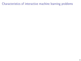
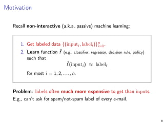
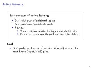
This document discusses the difference between non-interactive and interactive machine learning, detailing typical processes and applications for both. It highlights interactive machine learning scenarios such as medical treatment adaptation, website content selection, and spam filter improvement by using user feedback. The document also outlines challenges like sampling bias in active learning and methodologies for importance weighted active learning to ensure statistically consistent results.


![Framework for statistically consistent active learning
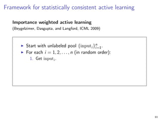
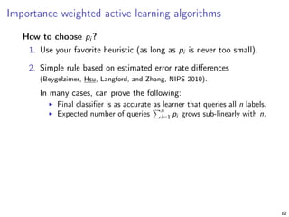
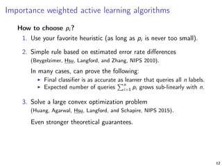
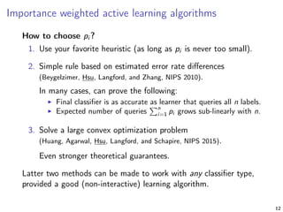
Importance weighted active learning
(Beygelzimer, Dasgupta, and Langford, ICML 2009)
Start with unlabeled pool {inputi }n
i=1.
For each i = 1, 2, . . . , n (in random order):
1. Get inputi .
2. Pick probability pi ∈ [0, 1], toss coin with P(heads) = pi .
11](https://image.slidesharecdn.com/nyaiinteractivelearningdanielhsu-160427230654/85/NYAI-Interactive-Machine-Learning-by-Daniel-Hsu-51-320.jpg)
![Framework for statistically consistent active learning
Importance weighted active learning
(Beygelzimer, Dasgupta, and Langford, ICML 2009)
Start with unlabeled pool {inputi }n
i=1.
For each i = 1, 2, . . . , n (in random order):
1. Get inputi .
2. Pick probability pi ∈ [0, 1], toss coin with P(heads) = pi .
3. If heads, query labeli , and include (inputi , labeli ) with
importance weight 1/pi in data set.
11](https://image.slidesharecdn.com/nyaiinteractivelearningdanielhsu-160427230654/85/NYAI-Interactive-Machine-Learning-by-Daniel-Hsu-52-320.jpg)
![Framework for statistically consistent active learning
Importance weighted active learning
(Beygelzimer, Dasgupta, and Langford, ICML 2009)
Start with unlabeled pool {inputi }n
i=1.
For each i = 1, 2, . . . , n (in random order):
1. Get inputi .
2. Pick probability pi ∈ [0, 1], toss coin with P(heads) = pi .
3. If heads, query labeli , and include (inputi , labeli ) with
importance weight 1/pi in data set.
Importance weight = “inverse propensity” that labeli is queried.
Used to account for sampling bias in error rate estimates.
11](https://image.slidesharecdn.com/nyaiinteractivelearningdanielhsu-160427230654/85/NYAI-Interactive-Machine-Learning-by-Daniel-Hsu-53-320.jpg)


![Contextual bandit learning
Protocol for contextual bandit learning:
For round t = 1, 2, . . . , T:
1. Observe contextt. [e.g., user profile]
14](https://image.slidesharecdn.com/nyaiinteractivelearningdanielhsu-160427230654/85/NYAI-Interactive-Machine-Learning-by-Daniel-Hsu-64-320.jpg)
![Contextual bandit learning
Protocol for contextual bandit learning:
For round t = 1, 2, . . . , T:
1. Observe contextt. [e.g., user profile]
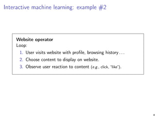
2. Choose actiont ∈ Actions. [e.g., display ad]
14](https://image.slidesharecdn.com/nyaiinteractivelearningdanielhsu-160427230654/85/NYAI-Interactive-Machine-Learning-by-Daniel-Hsu-65-320.jpg)
![Contextual bandit learning
Protocol for contextual bandit learning:
For round t = 1, 2, . . . , T:
1. Observe contextt. [e.g., user profile]
2. Choose actiont ∈ Actions. [e.g., display ad]
3. Collect rewardt(actiont) ∈ [0, 1]. [e.g., click or no-click]
14](https://image.slidesharecdn.com/nyaiinteractivelearningdanielhsu-160427230654/85/NYAI-Interactive-Machine-Learning-by-Daniel-Hsu-66-320.jpg)
![Contextual bandit learning
Protocol for contextual bandit learning:
For round t = 1, 2, . . . , T:
1. Observe contextt. [e.g., user profile]
2. Choose actiont ∈ Actions. [e.g., display ad]
3. Collect rewardt(actiont) ∈ [0, 1]. [e.g., click or no-click]
Goal: Choose actions that yield high reward.
14](https://image.slidesharecdn.com/nyaiinteractivelearningdanielhsu-160427230654/85/NYAI-Interactive-Machine-Learning-by-Daniel-Hsu-67-320.jpg)
![Contextual bandit learning
Protocol for contextual bandit learning:
For round t = 1, 2, . . . , T:
1. Observe contextt. [e.g., user profile]
2. Choose actiont ∈ Actions. [e.g., display ad]
3. Collect rewardt(actiont) ∈ [0, 1]. [e.g., click or no-click]
Goal: Choose actions that yield high reward.
Note: In round t, only observe reward for chosen actiont, and not
reward that you would’ve received if you’d chosen a different action.
14](https://image.slidesharecdn.com/nyaiinteractivelearningdanielhsu-160427230654/85/NYAI-Interactive-Machine-Learning-by-Daniel-Hsu-68-320.jpg)


![Framework for simultaneous exploration and exploitation
Initialize distribution W over some policies.
For t = 1, 2, . . . , T:
1. Observe contextt.
2. Randomly pick policy ˆπ ∼ W ,
choose ˆπ(contextt) ∈ Actions.
3. Collect rewardt(actiont) ∈ [0, 1],
update distribution W .
18](https://image.slidesharecdn.com/nyaiinteractivelearningdanielhsu-160427230654/85/NYAI-Interactive-Machine-Learning-by-Daniel-Hsu-88-320.jpg)
![Framework for simultaneous exploration and exploitation
Initialize distribution W over some policies.
For t = 1, 2, . . . , T:
1. Observe contextt.
2. Randomly pick policy ˆπ ∼ W ,
choose ˆπ(contextt) ∈ Actions.
3. Collect rewardt(actiont) ∈ [0, 1],
update distribution W .
Can use “inverse propensity” importance weights to account for
sampling bias when estimating expected rewards of policies.
18](https://image.slidesharecdn.com/nyaiinteractivelearningdanielhsu-160427230654/85/NYAI-Interactive-Machine-Learning-by-Daniel-Hsu-89-320.jpg)


![1_Introduction to Machine Learning [Autosaved].pptx](https://cdn.slidesharecdn.com/ss_thumbnails/1introductiontomachinelearningautosaved-250910004933-3913b711-thumbnail.jpg?width=640&height=640&fit=bounds)


