Activation functions are mathematical equations that determine the output of a neural network.

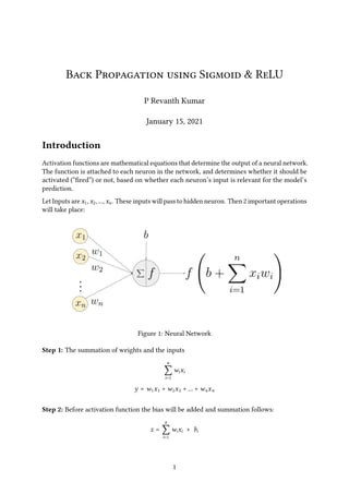
1. Back Propagation using Sigmoid & ReLU
P Revanth Kumar
January 15, 2021
Introduction
Activation functions are mathematical equations that determine the output of a neural network.
The function is attached to each neuron in the network, and determines whether it should be
activated (“fired”) or not, based on whether each neuron’s input is relevant for the model’s
prediction.
Let Inputs are 𝑥1, 𝑥2, ..., 𝑥𝑛. These inputs will pass to hidden neuron. Then 2 important operations
will take place:
Figure 1: Neural Network
Step 1: The summation of weights and the inputs
𝑛
∑
𝑖=1
𝑤𝑖𝑥𝑖
𝑦 = 𝑤1𝑥1 + 𝑤2𝑥2 + ... + 𝑤𝑛𝑥𝑛
Step 2: Before activation function the bias will be added and summation follows:
𝑧 =
𝑛
∑
𝑖=1
𝑤𝑖𝑥𝑖 + 𝑏𝑖
1

2. There are various kind of activation function. Here we will see some activation functions like:
1. Sigmoid
2. ReLu
1 Sigmoid Activation Function
This function basically used in Logistic Regression also.
𝜎(𝑥) =
1
1 + 𝑒−𝑧
where,
𝑧 =
𝑛
∑
𝑖=1
𝑤𝑖𝑥𝑖 + 𝑏𝑖
after transformation, the output transform the value between 0 and 1. Let the product be any
value +ve or -ve. Here, 0.5 is the threshold. If the value is lesser than 0.5 considered as 0. If the
value is greater than 0.5 considered as 1 (Neuron is activated).
Figure 2: Sigmoid function
1.1 Sigmoid function in Back Propagation
Whenever the weights are getting updated we need to find the derivative of the function.
𝜎(𝑥) =
1
1 + 𝑒−𝑧
differentiating sigmoid function with respect to x.
Now,
𝑑𝜎(𝑥)
𝑑𝑥
=
1
(1 + 𝑒−𝑥)2
· 𝑒−𝑥
2

3. =
𝑒−𝑥
(1 + 𝑒−𝑥)2
=
1
(1 + 𝑒−𝑥)
*
𝑒−𝑥
(1 + 𝑒−𝑥)
(sigmoid) (1-sigmoid)
∴
𝑑𝜎(𝑥)
𝑑𝑥
= 𝜎(𝑥)(1 − 𝜎(𝑥)).
The derivative of sigmoid activation function will lies between 0 to 0.25.
0 ≤
𝜕𝑓
𝜕𝑥
≤ 0.25
Figure 3: Derivative of sigmoid function
• Because of this the vanishing gradient problem occurs. Understand the weight’s update
𝑤𝑛𝑒𝑤 = 𝑤𝑜𝑙𝑑 − 𝜂
𝜕𝐿
𝜕𝑤
this will be calculated with the help of chain rule.
• Suppose, let us consider 3 derivatives over here 1𝑠𝑡
derivative is 0.25, 2𝑛𝑑
derivative is
0.10 and 3𝑟𝑑
derivative is 0.001 which will impact w.
• When multiply this number will give a very small value (0.000025). Now, let us put this
number in 𝜕𝐿
𝜕𝑤
and learning rate as 1, there will be a minor change in 𝑤𝑜𝑙𝑑 that means
𝑤𝑜𝑙𝑑 ≈ w𝑛𝑒𝑤. Because of this minor change it will take much time to converge in the
gradient descent curve.
Now, in order to vanish gradient problem how ReLu will help us, let us see...
3

4. 2 ReLU Activation Function
In ReLU activation function, suppose after particular operation
𝑧 =
𝑛
∑
𝑖=1
𝑤𝑖𝑥𝑖 + 𝑏𝑖
• If this particular function is pass to ReLu activation function then simple formula is
getting applied
𝑚𝑎𝑥 (0, 𝑧)
• Suppose if z is -ve then max (0,z) will be
−𝑣𝑒 𝑚𝑎𝑥 (0, −𝑣𝑒) = 0
• Suppose if z is +ve then max (0,z) will be
+𝑣𝑒 𝑚𝑎𝑥 (0, +𝑣𝑒) = +𝑣𝑒
• ReLu activation function is much more popular than sigmoid function.
Figure 4: ReLu function
4

5. 2.1 ReLU function in Back Propagation
Whenever we are doing back propagation the derivative of ReLu function will be 1.
The line y=x (from fig.4.) have an angle of 45𝑜
. The derivative of any positive value in the case
of ReLU function the output will be always 1 because tan 45𝑜
= 1.
Figure 5: Derivative of ReLu
• Derivative of a function 𝜕𝑓
𝜕𝑧
for ReLu will be always 0 or 1. Whenever derivative is
performed it will check z value.
⎧⎪⎪
⎨⎪⎪⎩
1 𝑧 > 0
0 𝑧 < 0
• Now, let us apply this formula in derivative.
Suppose,
𝑤𝑛𝑒𝑤 = 𝑤𝑜𝑙𝑑 − 𝜂
𝜕𝐿
𝜕𝑤
• Let the derivative be the chain rule it has 3 derivative values as 1 × 1 × 1 = 1 and learning
rate (𝜂) as 1. When these values are updated over 𝜕𝐿
𝜕𝑤
their will be little difference between
𝑤𝑜𝑙𝑑 and 𝑤𝑛𝑒𝑤.
• Now, this will not have the vanishing gradient problem and the weights will get converge.
• But their is small problem with ReLU function, actually fix by Leaky ReLU function.
• As the ReLU derivative will be either 0 or 1. Suppose in one of the derivative case 1×0×1
= 0.
• Now, 𝑤𝑜𝑙𝑑 = 𝑤𝑛𝑒𝑤 this basically create a "dead neuron". This means no process has been
taken place, in order to fix this Leaky ReLU function is used.
5

6. 2.2 Leaky ReLU
Leaky ReLUs are one attempt to fix the “dying ReLU” problem. Instead of the function being
zero when x < 0, a leaky ReLU will instead have a small negative slope of ( 0.01, or so)
Figure 6: Leaky ReLU activation function
⎧⎪⎪
⎨⎪⎪⎩
𝑧 𝑧 > 0
0.01 (𝑧) 𝑧 < 0
• Now, if we do the derivative with respect to z
𝜕(0.01)𝑧
𝜕𝑧
= 0.01 ; but it will not be = 0.
• This means we are solving "dead neuron" during the back propagation by using Leaky
ReLU.
• Suppose, in a neural network there are 100 neurons based on the training cycle if their is
a problem of deactivating or neurons getting dead then Leaky ReLU need to be applied.
*Note: In sigmoid the derivative will be always range between 0 to 0.25, in tanh it is al-
ways lessthan 1, but in ReLU either 0 or 1.
6