Return period computation, plotting position, Probability computation.

1. 1
Lecture -5
Statistical Method
Return Period computation and plotting position
The probability P of an event equaled to or exceeded is given by the
Weibull Formula (a simple empirical technique) as given below:
P = m /(N + 1 ) (5-1)
Where ,
m = entry of a given annual extreme series in
descending order of magnitude
N = number of years of record
(Return period), T = 1/ P = ( N + 1) / m
The exceedence probability of the event by using an empirical
formula is called plotting position. Such as Empirical formula,
equation- (5-1).

2. 2
Lecture -5(contd.)
Example 3-2
For a station A, the recorded annual 24 h maximum
rainfall are given in the table below (a) Estimate the 24 h
maximum rainfall with return periods of 13 and 50 years.
(b) What would be the probability of a rainfall of
magnitude equal to or exceeding 10 cm occurring in 24 h
at station A.
Year 1950 1951 1952 1953 1954 1955 1956 1957 1958 1959 1960 1961 1962
rainfall
(cm)
13.0 12.0 7.6 14.3 16.0 9.6 8.0 12.5 11.2 8.9 8.9 7.8 9.0
Year 1963 1964 1965 1966 1967 1968 1969 1970 1971
rainfall
(cm)
10.2 8.5 7.5 6.0 8.4 10.8 10.6 8.3 9.5

3. 3
Lecture -5(contd.)
Solution
Given,
24 h maximum rainfall in the table
To be calculated
(a) maximum rainfall with return periods 13 and 50
years and
(b) What would be the probability of a rainfall of
magnitude equal to or exceeding 10 cm
occurring in 24 h at station A.
We can calculate probability using Weibull Formula
P = m/ (N+1), where, m = entry in descending order

4. 4
The data given in the table be arranged them in descending
order.
Then the probability and recurrence intervals (Return period) has
been calculated as mentioned in the following table :
Lecture -5(contd.)
m Rainfall
(cm)
Probability
P =m/(N+1)
Return
Period,
T=1/P, years
m Rainfall
(cm)
Probability
P =m/(N+1)
Return
Period, T=1/P
(years)
1 16.0 0.043 23.00 12 9.0 0.522 1.92
2 14.3 0.087 11.50 13 8.9 - -
3 13 0.130 7.67 14 8.9 0.609 1.64
4 12.5 0.174 5.75 15 8.5 0.652 1.53
5 12.0 0.217 4.60 16 8.4 0.696 1.44
6 11.2 0.261 3.83 17 8.3 0.739 1.35
7 10.8 0.304 3.29 18 8.0 0.783 1.28
8 10.6 0.348 2.88 19 7.8 0.826 1.21
9 10.2 0.391 2.56 20 7.6 0.870 1.15
10 9.6 0.435 2.30 21 7.5 0.913 1.10
11 9.5 0.478 2.09 22 6.0 0.957 1.05

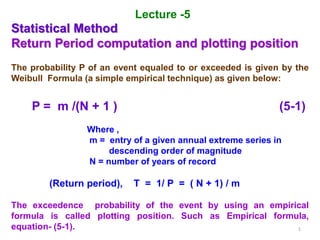
5. 5
•
••
•
•
•
•
•
•
•
••
••
••
•
•
•
1 10 100
Return Period, T in Years
Rainfallmagnitudeincm
19.0
18.0
14.0
13.0
12.0
7.0
6.0
5.0
Semi Log Paper
Figure: Rainfall vs Return Period
Now a graph is plotted between the rainfall magnitude and
the return period T on a semi log paper.
Lecture -5(contd.)
Graph represents the
relation between
rainfall and Return
period

6. 6
(When two or more magnitude are same (as m = 13 and 14
in above table) P is calculated for the largest m value of
the set.)
Lecture -5(contd.)
Return period T years Rainfall magnitude (cm)
13 14.55
50 18.0
From above graph
(a) maximum rainfall with return periods 13 and 50 years
(b) For rainfall 10 cm, from graph: T= 2.4 years and
probability, p = 1/T =1/2.4= 0.417

7. 7
Lecture -5(contd.)
Evaporation
Evaporation is the process in which a liquid changes to the
gaseous state at the free surface, below the boiling point through
the transfer of heat energy. The net escape of water molecules
from the liquid state to gaseous state constitutes evaporation.
Evaporation is a cooling process in that the latent heat of
vaporization (at about 585 cal/g of evaporated water) must be
provided by the water body.
The rate of vaporization is dependent on
 the vapor pressure at the water surface and air above
 air and water temperatures
 wind speed
 atmospheric pressure
 quality of water
 size of water body

8. 8
Lecture -5(contd.)
Dalton Law of evaporation
Vapor pressure
The rate of evaporation is proportional to the
difference between the saturation vapor
pressure at the water temperature, ew and the
actual vapor pressure in the air, ea is Dalton
Law of evaporation .Thus,
EL ∞ ( ew – ea)
i.e.
EL = C ( ew – ea)

9. 9
Lecture -5(contd.)
Where, EL = Lake or rate of evaporation(mm/day)
C = Constant
ew= vapor pressure at the water temp.(in mm of Hg)
ea = actual air pressure (in mm of Hg)
when,
ew= ea Evaporation continues and
ew > ea condensation
Evaporation from sea water is about 2 – 3 %
less than the fresh water.

10. 10
Lecture -5(contd.)
Measurement of Evaporation
It is utmost necessary to measure the evaporation for
planning and operation of reservoirs and irrigation
systems.
There are various methods to measure the water
evaporated from water surface : Here are three methods:
1. Evaporimeter data
2. Empirical evaporation equation
3. Analytical methods

11. 11
(i) Evaporimeters
The instruments by which evaporation is measured is
called evaporimeters (water containing pans)
The rate of evaporation from a pan or tank evaporimeter is
measured by the change in level of its free water surface. Several
types of automatic evaporation pans are in use. The water level in
such a pan is kept constant by releasing water into the pan from a
storage tank or by removing water from the pan when
precipitation occurs.
The amount of water added to, or removed from, the pan is
recorded. In some tanks or pans, the level of the water is also
recorded continuously by means of a float in the stilling well. The
float operates a recorder. The difference of water level in the pan
is the measure of water vapor.
Lecture -5(contd.)

12. 12
Lecture -5(contd.)
(2) Empirical evaporation equation
Mayer’s formula(1915) :
EL = KM (ew-ea) (1+ u9/16 ) (5-2)
Where
KM = Coefficient account for various factors.
Value = 0.36 for large deep water and
= 0.50 for small shallow waters
For
u9 = monthly mean wind velocity in km/h at about 9 m
above ground
EL , ew and ea

13. 13
Lecture -5(contd.)
3) Analytical methods of evaporation
estimation
The analytical methods for the determination
of evaporation is broadly classified into
three categories:
iii. mass-transfer method
i. Water- budget .method
ii. energy- balance method

14. 14
3.i Water – budget method
The water- budget method is the simplest and is also the least
reliable. Considering the daily average values for a lake, the
continuity equation is written as
P + Vis + Vig = Vos + Vog + EL + ∆S + TL (5-3)
Where,
P = daily precipitation
Vis = daily surface inflow into the lake
Vig = daily ground water inflow
Vos = daily surface outflow from the lake
Vog = daily seepage outflow
EL = daily lake evaporation
∆ S = increase in lake storage in a day
TL = daily transpiration loss
Lecture -5(contd.)

15. 15
Lecture -5(contd.)
The units of the equations are in volume (m3 ) or depth
(mm) over a reference area.
Then the above Eq-3 can be written as
EL = P + (Vis - Vos ) + (Vig - Vog) - ∆ S - TL (5-4)
b) Energy-budget method
The energy – budget method is an application of the law
of conservation of energy. The energy available for
evaporation is determined by considering the incoming
energy, outgoing energy and energy stored in water
body over a known time interval.

16. 16
Back radiation (Hb )
Reflected(rHc)
Heat loss to air (Ha)
Solar radiation (Hc )
Refracted r(1-Hc)
Heat flux into the gr.
(Hg )
Heat stored (Hs) Advection(Hi )
Evaporation, (He = р LEL )
Figure- 3 : Energy balance in a water body
Lecture -5(contd.)
Considering the water body as shown in the following
figure-3, the energy balance to the evaporating surface
in a period of one day is given by :
Hence Energy balance:
Hn = Ha + He + Hg + Hs + Hi (5-5)

17. 17
where,
Hn = net heat energy received by the water surface
= Hc ( 1 – r ) – Hb and
Hc (1- r) = incoming solar radiation into a surface of
reflection coefficient (albedo) r
Hb = back radiation(long wave) from body
Ha = sensible heat transfer from water surface to air
He = heat energy used up in evaporation
= р LEL
Here, р = density of water,
L = latent heat of evaporation, and
EL = Evaporation in mm per day
Lecture -5(contd.)

18. 18
Hg = heat flux into the ground
Hs = heat stored in water body
Hi = net heat conducted out of the system by water flow
(advected energy)
The unit for all the energy terms in above equation (5-5)
are in calories per square mm per day.
Lecture -5(contd.)

19. 19
Lecture -5(contd.)
Hs and Hi can be neglected If the time period are short.
All the terms above can either be measured or evaluated
indirectly except (Ha).
The sensible heat term Ha is estimated using Bowen’s ratio β
given by the expression :
β = Ha / р LEL = 6.1 x 10 - 4 x Pa (Tw - Ta)/(ew - ea) (5-6)
Where, Pa = atmospheric pressure in mm of mercury,
ew = saturated vapor pressure in mm of Hg
ea = actual vapor pressure of air in mm of Hg
Tw = temperature of water surface in 0 C and
Ta = temperature of air in 0 C.

20. 20
Lecture -5(contd.)
Hence from the above Eq-5
EL = Ha / β р L (5-7)
From equation (5-5), we find
Ha = Hn –( He + Hg + Hs + Hi )
Putting the value of Ha to equation (5-7)
EL = {Ha / (β рL)} = {Hn – ( He + Hg + Hs + Hi )}/ {β р L}

21. 21
Lecture -5(contd.)
Again, He = р LEL
β р LEL = Hn –( р LEL + Hg + Hs + Hi )
β р LEL + р LEL = Hn – ( Hg + Hs + Hi )
EL = {Hn – ( Hg + Hs + Hi ) }/{р L (β + 1)} (5-8)
Only 5% errors arises when use this equation
for less than 7 days.

22. 22
Lecture -5(contd.)
Example 5-3:
Determine the lake evapotranspiration for an open
water surface, if the net radiation is 300 W/m2 and the
air temperature 300C. The water surface temperature
is 450C. The atmospheric pressure of air 50 mm of Hg.
other information are given below:
The density of water: 1000kg/m3
Relative humidity : 75%
Latent heat, L = 2501 – 2.37 Ta (KJ/kg)
where, Ta = air temperature in 0C
Assume, Sensible heat, ground heat flux, heat stored
in water body and reflected/advected energy equal to
zero

23. 23
Solution
Given,
The density of water, р =1000kg/m3
Relative humidity: 75% and
Latent heat, L = 2501 – 2.37 Ta (KJ/kg)
where, Ta = air temperature in 0C = 30 0C
net heat radiation, Hn = 300 W/ m2
The density of water, ρ = 1000kg/m3
water temperature, Tw = 45 0C
Atmospheric pressure, Pa= 50 mm Hg
Lecture -5(contd.)

24. 24
Lecture -5(contd.)
Given (contd.) : Assume
Sensible heat, ground heat flux, heat stored in
water body and reflected/advected energy
equal to zero i.e
Sensible heat, Ha = 0
Ground heat flux, Hg = 0
Heat stored in water body, Hs = 0 and
Reflected/advected energy, Hi = 0
We know from equation (5-8)
EL = Lake Evapotranspiration mm/day
EL = [Hn –Hg –Hs -Hi] / ρL(1+)

25. 25
Lecture -5(contd.)
Again from Bowen’s ratio β given by the
expression
β = Ha / р LEL = 6.1 x 10 -4 x Pa ( Tw- Ta)/ (ew – ea) (5-9)
Where, Pa = atmospheric pressure = 50 mm of Hg
ew = saturated vapor pressure in mm of Hg
From table 3-3
for Tw = 450C = 71.20 mm of Hg
ea = Relative humidity × ew = 0.75 ×71.20
=53.40 mm of Hg

26. 26
Table 3.3:
Slope of the saturation vapor pressure vs temperature curve at
the mean air temperature in mm of mercury per 0C
Temperature 0C Saturation vapor pressure (ew)
in mm of Hg
A
(mm / 0C )
15 12.79 0.80
17.5 15.00 0.85
20 17.54 1.05
22.5 20.44 1.24
25 23.76 1.40
27.5 27.54 1.61
30 31.82 1.85
32.5 36.68 2.07
35 42.81 2.35
37. 48.36 2.62
40 55.32 2.95
45 71.20 3.66

27. 27
Lecture -5(contd.)
Now putting the concerned values in equation (5-9),
β = Ha / р LEL = 6.1 x 10 -4 x 50 ( 45- 30)/ (71.20 – 53.40)
= 0.0257
L = 2501 – 2.37 ×30 (KJ/kg) = 2430 KJ/kg
Putting the concerned values in equation(5-8)
EL = [Hn –Hg –Hs -Hi] / ρL(1+)
EL = [Hn –0 - 0 -0] / [1000×2430 (1+0.0257]
EL = [300 –0 - 0 -0] / [1000×2430 (1+0.0257]
= 1.204 × 10-4 m/day
= 0.12 mm/day Ans.