wireframe.ppt

Pankaj Chhabra CAD/CAM
Wireframe Modeling
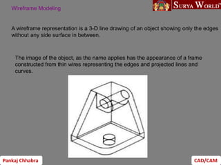
A wireframe representation is a 3-D line drawing of an object showing only the edges
without any side surface in between.
The image of the object, as the name applies has the appearance of a frame
constructed from thin wires representing the edges and projected lines and
curves.

A computer representation of a wire-frame structure consists essentially of two
types of information:
• The first is termed metric or geometric data which relate to the 3D coordinate
positions of the wire-frame node’ points in space.
Wireframe Modeling
• The second is concerned with the connectivity or topological data, which
relate pairs of points together as edges.
 Basic wire-frame entities can be divided into analytic and synthetic entities.
Analytic entities :
Points Lines Arc Circles
Synthetic entities:
Cubic curves Bezier curves B-spline curves

Wire-frame model
• Example : tetrahedron

Wireframe Modeling
Limitations
• From the point of view of engineering Applications, it is not possible to
calculate volume and mass properties of a design
• In the wireframe representation, the virtual edges (profile) are not
usually provided.
 (for example, a cylinder is represented by three edges, that is, two circles
and one straight line)
• The creation of wireframe models usually involves more user effort to
input necessary information than that of solid models, especially for
large and complex parts.

Disadvantages of wire-frame
• Tend to be not realistic
• Ambiguity
– complex model difficult to interpret.
What does this object look like?

Which object does the previous wire-frame represent?
The use of shading and hidden surface removal technique can improve the
rendition.

• Does not allow for use of photo realistic rendering
tools. *(some software capable of hidden line
removal on limited basis).
• No ability to determine computationally information
on mass properties (e.g. volume, mass, moment etc)
and line of intersect between two faces of
intersecting models.
• No guarantee that the model definition is correct,
complete or manufacturable.

Advantages of wire-frame
• Most economical in term of time and memory
requirement.
• Used to model solid object.
• Often used for previewing objects in an
interactive scenario.

Analytic curves are well defined.
However objects will benefit from the ability to alter
them.
e.g., car body, fuselage, wings, turbine blades etc.
Parametric representation of curves
allowing the ability to control the shape of
the curves have been developed as a
solution to this problem.

Analytical Curves
1- Non-parametric representation analytical curves
aX
Y
b
Y
a
X
R
Y
X
c
mX
Y
4
1
2
2
2
2
2
2
2
2







Line
Circle
Ellipse
Parabola
• Although non-parametric representations of curve equations are used in some cases,
they are not in general suitable for CAD because:
• The equation is dependent on the choice of the coordinate system
• Implicit equations must be solved simultaneously to determine points on the curve,
inconvenient process.
• If the curve is to be displayed as a series of points or straight line segments, the
computations involved could be extensive.

Analytical Curves
2- Parametric representation of analytical curves
In parametric representation, each point on a curve is expressed as a function
of a parameter u. The parameter acts as a local coordinate for points on the
curve.
T
T
u
z
u
y
u
x
z
y
x
u
P )]
(
)
(
)
(
[
]
[
)
( 

For 3D Curve
max
min u
u
u 

• The parametric curve is bounded by two parametric values Umin and Umax
• It is convenient to normalize the parametric variable u to have the limits 0 and 1.

Analytical Curves
1- Lines
• A line connecting two points P1 and P2.
• Define a parameter u such that it has the values 0 and 1 at P1 and P2
respectively
)
(
1
0
)
(
)
(
1
0
)
(
1
2
1
1
2
1
1
2
1
1
2
1
z
z
u
z
z
u
y
y
u
y
y
x
x
u
x
x
u
P
P
u
P
P
















Vector form
Scalar form
The above equation defines a line bounded by the endpoints P1 and P2 whose
associated parametric value are 0 and 1

Analytical Curves
2- Circles
• The basic parametric equation of a circle can be written as
For circle in XY plane, the parameter u is the angle measured from the X-axis to
any point P on the circle.
c
c
c
z
z
u
u
R
y
y
u
R
x
x








2
0
sin
cos

Analytical Curves
3- Circular Arcs
• Circular arcs are considered a special case of circles. A circular arc parametric
equation is given as
Where us and ue are the starting and ending angles of the arc respectively
c
e
s
c
c
z
z
u
u
u
u
R
y
y
u
R
x
x







sin
cos

Synthesis Curves
Curves that are constructed by many curve
segments are called Synthesis Curves
• Analytic curves are not sufficient to meet
geometric design requirements of
mechanical parts
• Products such as car bodies, airplanes,
propeller blades, etc. are a few examples
that require free-form or synthetic curves
and surfaces

•Control points
•Axis independence
•Local and Global Control
•Variation diminishing property
•Versatility
•Order of continuity
Curves
•Control points

•Axis independence
•Local and Global Control

•Variation diminishing property

•Order of continuity
Continuity- how smooth are the curves at the point
of junction of two curves.
Three types:
C0, C1, and C2.
C0-The two curves are simply connected. Gradient
and curvature may be different.

Synthesis Curves
1- Interpolation
Finding an arbitrary curve that fits (passes through) a set of given points. This
problem is encountered, for example, when trying to fit a curve to a set of
experimental values.
Types of interpolation techniques:
• Lagrange polynomial
• Parametric cubic (Hermite)
Parametric cubic
• Mathematical approaches to the representation of curves in CAD can be
based on either
• Interpolation
• Approximation

Synthesis Curves
2- Approximation
Approximation approaches to the representation of curves provide a smooth
shape that approximates the original points, without exactly passing
through all of them.
Two approximation methods are used:
• Bezier Curves
• B-spline Curves
Bezier Curves
B-spline curves
 If the problem of curve design is a problem of data fitting, the classic
interpolation solutions are used.
 If the problem is dealing with free form design with smooth shapes,
approximation methods are used.

Representation of entities (Bezier)
• .
• P.Bezier, an employee of the French
auto company Renault, suggested a
new form of curve equation and used
it in Renault’s surface modeling
system, UNISURF.
– The curve is defined by the vertices of a
polygon that enclose the resulting
curve.

– The effects of the vertices are weighted by
the corresponding blending functions and
blended as in the Hermite curve.
• The resulting function has the
following properties:
– The curve passes through the first and the
last vertex of the polygon
– The tangent vector at the starting point of
the curve has same direction as the first
segment of the polygon (Figure 25) .
Similarly the last segment of the polygon
gives the slope of the tangent vector at the
ending point.

Figure 25

BLENDING FUNCTION



n
i
i
i x
P
a
x
f
0
, )
(
)
(

• Bezier curves are based on approximation
techniques in comparison to Hermite
curves which are based on interpolation
techniques.
• In Bezier, the curves do not pass through
all the given points except the first and
last control point.
• Does not require the first-order derivatives
and the shape of the curve is controlled by
control points.

Synthesis Curves
2- Bezier Curves
Given n+1 control points, P0, P1, P2, ….., Pn, the Bezier curve is defined by the
following polynomial of degree n
1
0
)
(
)
(
0
, 

 

u
P
u
B
u
P
n
i
i
n
i

)!
(
!
!
)
,
(
)
1
(
)
,
(
)
(
,
i
n
i
n
i
n
C
u
u
i
n
C
u
B i
n
i
n
i



 
where
P(u) is any point on the curve
Pi is a control point, Pi = [xi yi zi]T
Bi,n are polynomials (serves as basis function for the Bezier Curve)
where
Synthesis Curves
2- Bezier Curves
In evulating these expressions
00 = 1
0! =1
C(n,0) = C(n,n)=1 when u and i are 0

Synthesis Curves
2- Bezier Curves
The above equation can be expanded to give
n
n
n
n
n
n
n
u
P
u
u
n
n
C
P
u
u
n
C
P
u
u
n
C
P
u
P
u
P















)
1
(
)
1
,
(
..........
)
1
(
)
2
,
(
)
1
(
)
1
,
(
)
1
(
)
(
1
1
2
2
2
1
1
0
0 ≤ u ≤ 1

Hermite Spline
• Say the user provides
• A cubic spline has degree 3, and is of the form:
– For some constants a, b, c and d derived from the
control points, but how?
• We have constraints:
– The curve must pass through x0 when u=0
– The derivative must be x’0 when u=0
– The curve must pass through x1 when u=1
– The derivative must be x’1 when u=1
d
cu
bu
au
x 


 2
3
1
0
1
0 ,
,
, x
x
x
x 


0
y
1
y
2
y
3
y
4
y
5
y
6
y
)
(
0 u
Y )
(u
Y
)
(
5 u
Y
u

6

u

0

u




















1
)
1
(
)
1
(
1
≡
3
2
)
1
(
≡
)
0
(
≡
)
1
(
≡
)
0
(
i
i
i
i
i
i
i
i
i
i
i
i
i
i
i
i
i
D
d
c
b
Y
D
b
Y
y
d
c
b
a
Y
y
a
Y
5
,...,
0
1
0
)
(
P 3
2
i







i
u
u
d
u
c
u
b
a
u i
i
i
i
1
1
1
1
)
(
2
2
)
(
3














i
i
i
i
i
i
i
i
i
i
i
i
i
i
D
D
y
y
d
D
D
y
y
c
D
b
y
a
1 2 3 4 5
Hermite Interpolation

Hermite Spline
A Hermite spline is a curve for which the user provides:
– The endpoints of the curve
– The parametric derivatives of the curve at the
endpoints
• The parametric derivatives are dx/dt, dy/dt, dz/dt
– That is enough to define a cubic Hermite spline, more
derivatives are required for higher order curves

Hermite Spline
• Solving for the unknowns gives:
• Rearranging gives:
0
0
0
1
0
1
0
1
0
1
2
3
3
2
2
x
d
x
c
x
x
x
x
b
x
x
x
x
a
















)
2
(
)
(
x
)
1
3
2
(
)
3
2
(
2
3
0
2
3
1
2
3
0
2
3
1
t
t
t
x
t
t
t
t
x
t
t
x
x













 

































1
0
1
2
1
0
0
1
1
1
0
3
2
0
0
3
2
2
3
0
1
0
1
u
u
u
x
x
x
x
x
or

Hermite curves in 2D and 3D
• We have defined only 1D splines:
x = f(t:x0,x1,x’0,x’1)
• For higher dimensions, define the control
points in higher dimensions (that is, as
vectors)

























































1
0
1
2
1
0
0
1
1
1
0
3
2
0
0
3
2
2
3
0
1
0
1
0
1
0
1
0
1
0
1
u
u
u
z
z
z
z
y
y
y
y
x
x
x
x
z
y
x

wireframe.ppt

Recommended

Recommended

More Related Content

Similar to wireframe.ppt

Similar to wireframe.ppt (20)

More from PankajChhabra31

More from PankajChhabra31 (7)

Recently uploaded

Recently uploaded (20)

wireframe.ppt