1. Bezier Curves with Quadratic Control Point
Interpolations
Nicolas I. Miguel
June 1, 2016
1 Introduction
Bezier curves are curves that have many applications, from car contour design
to font recognition1
. The curves are exact sections of many parabolas and
conics, and are the result of many linear interpolations/line fittings, which are
correlated with the degree of the curve. Furthermore, the curves have control
points that define many of the aspects of the curve, such as the degree of said
curve. In addition, Bezier curves are essentially parametric equations.
Throughout the last quarter, I have focused on Bezier curves that solely had
linear interpolations. That is, the connections between different control points
would be linear. In this paper, I will be exploring Bezier curves with quadratic
interpolations, where the connections between control points are in quadratic
form, instead of linear. The driving question behind this analysis is: How does
the degree of the function of a Bezier curve change depending on the degree of
interpolation?
From my last quarter papers, we can remember that a Bezier curve with n
original control points will have a degree of n − 1. This was only tested with
Bezier curves that utilized linear interpolations, therefore, I don’t know if this
rule will hold for Bezier curves that utilize quadratic interpolations. Therefore,
the goal of this project is to find if there is a rule which allows you to find the
degree of a Bezier curve depending on the number of control points and the
degree of the interpolation.
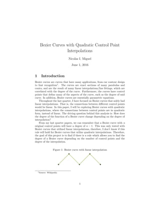
Figure 1: Bezier curve with linear interpolation
1Source: Wikipedia
1

2. Figure 2: Bezier curve with quadratic interpolation
2 Curves with 3 control points
We start by observing a Bezier curve with 3 control points. With normal linear
interpolation, the skeleton of the curve (that is, the control points and the
connections between those original control points) looks like this:
However, we are looking at quadratic interpolation. Thus, the path between
two control points will have to be quadratic. To define these parabolas, we’ll
consider P1 (the original control point farthest to the left) as the vertex for a
parabola which goes through P2 (the original control point to the immediate
right of P1). Furthermore, we’ll consider P2 to be the vertex for a parabola
which goes through P3 (the point to the right of P2). We’ll have that:
P1 = (−2, 0)
P2 = (0, 2)
P3 = (2, 0)
We consider the first interpolation, which is a parabola where P1 is the vertex,
and P2 is a point the parabola goes through:
y = a(x − h)2
+ k
y = a(x − (−2))2
+ 0
y = a(x + 2)2
2 = 4a
a =
1
2
y =
1
2
(x + 2)2
2

3. We repeat a similar process and get that the parabola that has P2 as a
vertex and goes through P3 is of the form: y = −1
2 x2
+ 2. This looks like so
(note that I’ve restricted the domain of both parabolas so that they stay within
the bounds of the skeleton):
Now we need to find the parametric equations for the two points that move
along the two paths. We’ll call these points L1, which travels on the first path,
and L2, which travels on the second path. Starting with L1, we see that at
time t=0, L1 will be at (−2, 0), and at t=1, L1 will be at (0, 2). Thus, we
find that xL1(t) = 2t − 2, since at t = 0, L1’s x-coordinate is at -2 and at
t = 1 it is at 0. However, to find the y-coordinate we need to manipulate the
points a bit differently. Instead of only dealing with L1 at t=0 or t=1, we also
need to consider where L1 is at t=-1. This is because the y-coordinate of the
point does not stay at the same rate, rather, the rate changes because the path
is a parabola. Thus, we need three points to calculate the L1’s y-coordinate
parametric equation. We already know that at t = 0, y=0 and at t = 1, y=2.
However, since this is a parabola, we will consider that at t = −1, L1 was at the
point (−4, 2), thus at t = −1, y = 2. The following graphic best details what I
am doing:
Thus, we see that we have three points in the form (t, y): (−1, 2), (0, 0), and
(1, 2). Naturally, we observe that (0, 0) is the vertex, thus, we solve like any
3

4. other parabola:
y = a(t + h)2
+ k
y = a(t + 0)2
+ 0
y = at2
2 = a(−1)2
2 = a
y = 2t2
Thus, we have parametrics for L1.
L1 = (2t − 2, 2t2
)
We repeat the same process for L2, proposing that at t = −1, L2 is at (−2, 0),
like so:
We find that xL2(t) = 2t, and after setting up three points in the form
(t, y) ((−1, 0), (0, 2), and (1, 0), where (0, 2) is the vertex), we find that the
y-coordinate is given by:
y = a(t − h)2
+ k
y = at2
+ 2
0 = a + 2
a = −2
y = −2t2
+ 2
We have the parametrics for L2.
L2 = (2t, 2 − 2t2
)
Now that we have the two secondary control points, our curve skeleton looks
like this:
4

5. L1 is the red point on the left path, and L2 is the red point on the right path.
The next step we take is finding an equation for the parabolic path between
L1 and L2. Let’s consider that L1 is the vertex, and L2 is a point on that
parabola. Once again, we set up:
y = a(x − h)2
+ k
y = a(x − xL1)2
+ yL1
y = a(x − 2t + 2)2
+ 2t2
yL2 = a(xL2 − 2t + 2)2
+ 2t2
2 − 2t2
= a(2t − 2t + 2)2
+ 2t2
y =
1
2
− t2
(x − 2t + 2)2
+ 2t2
Once we find the equation of the path, we have (in red):
The final step is to figure out the parametric equation for the final control
point. The point, which we’ll call R, will travel along the red path, which we
just figured out. At t = 0, R = (xL1, yL1). At t = 1, R = (xL2, yL2). Figuring
out the parametric equation for xR is simple enough. We know that x goes from
-2 to 2 in 1 second, thus: xR(t) = 4t − 2. For the parametric equation for the
5

6. y-coordinate, all we have to do is plug in xR(t) for ‘x’ in the equation of the red
path (y = 1
2 − t2
(x − 2t + 2)2
+ 2t2
). We get:
y =
1
2
− t2
((4t − 2) − 2t + 2)2
+ 2t2
Ultimately, the parametric equations for the final control point R are:
(4t − 2,
1
2
− t2
((4t − 2) − 2t + 2)2
+ 2t2
)
The skeleton is finally complete, and the curve is traced out by R (the blue
point):
Now we solve for the path traced out by R by solving for t in terms of x and
then replacing that for the t in the parametric equation for y, like so:
x = 4t − 2
t =
x + 2
4
y =
1
2
−
x + 2
4
2
4
x + 2
4
− 2 − 2
x + 2
4
+ 2
2
+ 2
x + 2
4
2
y = −
1
64
x4
−
1
8
x3
−
1
8
x2
+
1
2
x +
3
4
The function that results is of degree 4, which is the degree of a linearly-
interpolated 3-point Bezier curve (2) multiplied by 2. Here we observe the
graph of the Bezier curve, which is in orange:
6

7. 3 Curve with 4 control points
We repeat the same process as before, setting up a skeleton and solving for each
set of respective control points. Ultimately, we get a path traced out by the
blue point:
The final path looks like this (in blue):
The function of the path is of degree 6, which is the degree of the linearly-
interpolated 4-point Bezier curve (3) multiplied by 2.
4 Conclusion
With the two examples we have been given, we see that the final degree of the
curve is the degree of the normal Bezier curve multiplied by 2, which happens
7

8. to be the degree of the paths between the control points. Let’s consider the
paths between the control points in the curve skeletons. These are the green
paths in the diagrams, or the first set of interpolations. Consider looking at
them as individual Bezier curves. To get a quadratic Bezier curve with normal,
linear-interpolation, we would need 3 control points. Consider the diagram with
the 4 control points, above. There are three green paths, which connect P1,
P2, P3, and P4, like so:
Here, the black points and path become the first control points and linear in-
terpolation, and the green path and points become the second control points
and interpolations. Considering the original quadratically-interpolated 4-point
curve as part of a composition of normally interpolated 3-point curves allows us
to view how the curve operates. We see that we end up with 7 control points,
meaning that the final Bezier curve ends up with degree 6 (the blue function).
We can extend this to interpolations of any degree k between control points.
Ultimately, if you have n control points, p paths between those original control
points, and interpolation of degree k, we can write a rule for the degree of the
resulting Bezier curve (d):
d = ((k + 1) (p) − (n − 2)) − 1
Getting this answer is quite simple. We know that if we have a Bezier curve
with k degree interpolation, and p paths between the first control points, then
it can be split into p sections with k + 1 control points per section. With the 4-
point 2-degree interpolation Bezier curve, we see that the curve has 3 quadratic
paths, each quadratic path requiring 3 linearly-interpolated control points to
form. Thus, we would have a total of 3 ∗ 3 =9 control points. However, some of
these control points would serve as control points for two different paths, since
we’re treating the Bezier curve skeleton (the green paths) as an amalgam of
lower-degree Bezier curves. More specifically, of all the original control points
(the points directly on the green paths), only the outside two, or farthest left
and right points, are not functioning as control points simultaneously for two
different curves. Thus, we end up getting that the total control points for
the curve, if it were linearly interpolated, would be ((k + 1) (p) − (n − 2)). In
this case, it calculates out to 7 total control points, and with any linearly-
interpolated Bezier curve, that would give a curve of degree 7-1=6.
In conclusion, we see that Bezier curves can have many interesting patterns
when varying and modifying some of the “rules” of said Bezier curves, in this
case changing the control point interpolation from linear to quadratic.
8