The document discusses different location modeling techniques to determine the optimal location for a new plant given the locations of existing facilities. It presents the simple median model, factor rating method, and break-even analysis. The simple median model is illustrated using a network of 4 existing facilities (F1-F4) where the new plant needs to supply raw materials. It determines the optimal location for the new plant as x=20, y=40 by finding the median load and corresponding x- and y-coordinates. The factor rating method and break-even analysis are also demonstrated through examples to select the best location among alternatives based on important factors and production volume ranges.

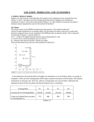
1. LOCATION MODELLING AND ECONOMICS
1. SIMPLE MEDIAN MODEL
Suppose we want to locate a new plant that will annually receive shipments of raw materials from two
sources: F1 and F2. The plant will create finished goods that must be shipped to two distribution
warehouses, F3 and F4. Given these four facilities (Figure 2.1), where should we locate the new plant to
minimize annual transportation costs for this network of facilities?
The Model
The simple median model (SMM) can help answer this question. This model considers the
volume of loads transported on rectangular paths. All movements are made in east-west or north-south
directions; diagonal moves are not considered. The SMM provides an optimal solution. This is discussed
with the help of Figure 2.1 and the Table 2.2.
Let Li = Loads to be shipped annually between each existing facility Fi, and
Ci= Cost to move a load one distance unit to or from Fi.
Di = Distance units between facility Fi and the new plant.
Then, the total transit cost is the sum of the products CiLiDifor all i.
A new plant has to be located which will supply raw materials to a set of existing plants in a group of
companies. There are four existing plants which require material movement with new plant. The material
transported (in tons) per year from new plant to existing plants are as given below. Determine the
optimum location for the new plant such that the distance move is minimum.
Existing Plant F1 F2 F3 F4
Location (X,Y) of Existing Plants (20,30) (10,40) (30,.50) (40,60)
Loads to be shifted from new plant 755 900 450 500
to existing plants, Li
TABLE 2.2

2. The SMM model consists in finding the X0,Y0 co-ordinates of the new plant that result in minimum
transportation costs. We follow three steps:
1. Identify the median value of the Loads moved
2.Find the the x-co-ordinate of the new facility that sends or receives the median load
3. Find the y-coordinate of the new facility that sends or receives the median load
The x,y co-ordinate found in steps 2 and 3 define the new plants location.
(i) Identify the median load
The total number of loads moved to and from the new plant will be ∑ Li =755+900+450+500 = 2605. If
we think of each load individually and number them from 1 to 2605, then the median load number is the “
middle” number- that is , number for which the same number of loads falls above and below. For 2605
loads the median load number is 1303 . If the total number of loads were even we consider both „middle
„ numbers.
(ii) Find the x – coordinate of the median load
First we consider movement of loads in the x-direction.
Beginning at the origin of Figure 2.1 and moving to the right along the x-axis, observe the number of
loads moved to or from existing facilities. Loads 1-900 are shipped by F2 from location x = 10. Loads
901-1,655 are shipped by F1 from x = 20. Since the median load falls in the interval 901-1,655, x = 20
is the desired x-coordinate location for the new plant.
(ii) Find the y – coordinate of the median load
Now consider the y-direction of load movements. Begin at
the origin of Figure 2.1 and move upward along the y-axis. Movements in the y direction begin with
loads 1-755 being shipped by F1 from location y = 30. Loads 756-1,655 are shipped by F2 from
location y = 40. Since the median load falls, in the interval 756-1,655, y = 40 is the desired ycoordinate
for the new plant.
• The optimal plant location, x = 20 and y = 40, results in minimizing annual transportation costs for this
network of facilities. The calculation is shown in Table 2.4.
Remarks:
• First, we have considered the case in which only one new facility is to be added.
• Second, we have assumed that any point in x-y coordinate system is an eligible point for locating the
new facility. The model does not consider road availability, physical terrain, population densities, or
any other considerations.

3. 2. Factor Rating Method
The process of selecting a new facility location involves a series of following steps:
1. Identify the important location factors.
2. Rate each factor according to its relative importance, i.e., higher the ratings is indicative
of prominent factor.
3. Assign each location according to the merits of the location for each factor.
4. Calculate the rating for each location by multiplying factor assigned to each location with
basic factors considered.
5. Find the sum of product calculated for each factor and select best location having highest
total score.
ILLUSTRATION 1: Let us assume that a new medical facility, Health-care, is to be
located in Delhi. The location factors, factor rating and scores for two potential sites are
shown in the following table. Which is the best location based on factor rating method?
The total score for location 2 is higher than that of location 1. Hence location 2, is the best
choice.

4. 3..Break-even Analysis
Break even analysis implies that at some point in the operations, total revenue equals total cost.
Break even analysis is concerned with finding the point at which revenues and costs agree
exactly. It is called „Break-even Point‟. The Fig. 4.3 portrays the Break Even Chart:
Break even point is the volume of output at which neither a profit is made nor a loss is incurred.
Plotting the break even chart for each location can make economic comparisons of locations.
This will be helpful in identifying the range of production volume over which location can be
selected.
ILLUSTRATION 5: Potential locations X, Y and Z have the cost structures shown below.
The ABC company has a demand of 1,30,000 units of a new product. Three potential
locations X, Y and Z having following cost structures shown are available. Select which
location is to be selected and also identify the volume ranges where each location is suited?
LOCATION X LOCATION Y LOCATION Z
FIXED COST Rs. 150,000 Rs. 350,00 Rs. 950,000
VARIABLE COST Rs. 10 Rs. 8 Rs. 6
SOLUTION: Solve for the crossover between X and Y:
10X + 150,000 = 8X + 350,000
2X = 200,000
X = 100,000 units
Solve for the crossover between Y and Z:
8X + 350,000 = 6X + 950,000
2X = 600,000
X = 300,000 units
Therefore, at a volume of 1,30,000 units, Y is the appropriate strategy.

5. From the graph (Fig. 4.4) we can interpret that location X is suitable up to 100,000 units,
location Y is suitable up to between 100,000 to 300,000 units and location Z is suitable if the
demand is more than 300,000 units.
LOCATIONAL ECONOMICS
An ideal location is one which results in lowest production cost and least distribution cost per unit.
These costs are influenced by a number of factors as discussed earlier. The various costs which
decide locational economy are those of land, building, equipment, labour, material, etc. Other factors
like community attitude, community facilities and housing facilities will also influence the selection
of best location. Economic analysis is carried out to decide as to which locate best location.
The following illustration will clarify the method of evaluation of best layout selection.
ILLUSTRATION 6: From the following data select the most advantageous location for
setting a plant for making transistor radios.