This midterm report summarizes progress on developing a program to generate cohesive zone models (CZM) using Python. The program has successfully generated CZM for basic, single-crack, and single-inclusion models. However, challenges remain in handling more complex multi-crack models. The report proposes addressing this by changing to an object-oriented structure and representing cracks as a tree to properly model crack junctions and updates to elements. Future work will focus on implementing this tree structure in Python while maintaining efficiency.
1. Network Team of Rock Damage Modeling and Energy Geostorage Simulation
Midterm Report: Benchmark Joint Elements, CZM and XFEM
Jianming Zeng
Introduction:
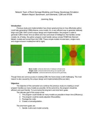
Previous study and implementation has shown great promise on how effectively python
could help generating CZM(cohesive zone model). It’s a very efficient way to generate relatively
large size CZM. With current unique design and implementation, the program is able to
generate CZM in linear time as before and has some level of intelligence that handles similar
models. As of today, the python program could handle various simple FEM(Finite Element
Model) models and turned them into CZM. These simple models include basic, single-crack,
and single-inclusion models(from left to right).
Basic model: cohesive elements in between all elements
Single crack: cohesive elements along one specific path
Single inclusion: cohesive elements around some geometry
Though there are some success in creating CZM, the future study is still challenging. The main
reason is also caused by the unique design and implementation(Discuss later).
Objective:
The objective of this semester is to continue the previous study on creating a smart
program handles as many models as possible. At the same time, the program should be
efficient and user-friendly. To summarize the long term and short term goals:
The ultimate goal of this study is that:
1. The program could handle as many models as possible in linear time (Efficiency).
2. The program could be easily adjusted (Reusability).
3. Package the code.
4. Create a manual/guideline .
The short term goals are:
1. Handle multi-crack model correctly.
2. 2. Change data structure (Object-oriented).
3. Describe elements behavior(wrt abaqus) on shared edges.
Theory:
Correctness and efficiency are the two key factors to be considered when implementing,
and efficiency should be considered before correctness. Why? For example, there are many
ways to calculate the distance between two points. But as we all know the shortest distance
between them is always the Euclidean one. There is always a upper time limit on how fast a
program could be. And therefore, one should always aims for the best complexity during the
implementation process.
In the above chart, it describes most of the complexity in computation. Letter “n” stands for the
size of the data or input. Depends on the type of calculation process and input size, calculation
time could have a significant difference. Though the input size is not under control, calculation
process is something we could make a difference. In a file I/O problem, the best time complexity
one could achieve is linear. The reason is because retrieving information from an input file and
write information to a file line by line takes as many time as the number of lines inside a file. In
other words, if there are 10 lines information within a file we want, the best we could do in this
case is to read line by line, or 10 lines, so that we get information from every line. And therefore,
if we do nothing, just reading information from file and put it back to the file, it takes O(n) + O(n),
or O(n). That is the upper limit performance we could achieve in this problem, and that is the
optimization we should aim for when start implementing.
Another useful theory in this task is graph theory. When constructing a FEM, abaqus
stores the model information in an inp file. This inp file contains two major parts. The geometry
information such as parts, nodes, and elements. And the physical property part controls any
other parameters. The cohesive element insertion is mostly geometrical alteration and abaqus
3. inp file doesn’t define any pairwise element relationship. Therefore graph theory is the best suit
for this task when storing data. Considering
the follow graph:
In abaqus, node is given by its coordinate
and element is made of the nodes ID that define
it(example to the above right). This tells very
little information where to put cohesive zone
elements, and hence searching for the right
place to put cohesive zone can be very
expensive. A naive approach is described in the pseudo:
For element in elements:
For node1 in element:
For node2 in element and node2 != node1:
Edge = (node1, node2)
If edge has neighbour:
Add cohesive elements
4. While this is only a simple version, we can tell is a very bad implementation. For loop is very
costly in term of time optimization. This naive approach constantly visits the same information
over and over again. With small data size the complexity may still look considerably good. But
time complexity grows exponentially in this model. One significant improvement is described by
graph theory. Like the following sketch, we could establish some sort of relationship between
nodes and elements. This implementation could decrease the number of revisit time to achieve
time optimization. In other words, with additional information, we could use a lot less for loop. A
possible pseudo as followed:
For edge in graph:
If elements[edge] contains two edges:
Add cohesive elements:
The actual implementation is more complicated but this set-up only requires one for loop and
therefore O(n).
Object Oriented Programming(OOP) and Data Structure:
5. OOP and data structure offer many options when completing the task. For the sake of
better structure, OOP should be used in
implementing the addition process of cohesive zone
elements. This setup gives a more precise
implementation of the graph theory. Node object
class has coordinate as local variables. And
Element object includes the node’s ID that define it.
Element Set, Node Set and Cohesive Zone Set
objects are optional because it doesn’t change the
geometry with or with putting nodes or elements
into set. So theses objects could be inserted into a
list or array for the same purpose. The graph to the
left is an example of how list or array performs in
term of different operations. Same graphs could be
found online for set and dictionary(hashmap). In
order to keep time complexity and space complexity
as small as possible, one should choose data
structure wisely. For example, list or array is one of
the best options for storing information in order and
set is best for data comparison. After all, list, set
and dictionary could build up the best solution for storing data in general.
Challenge:
The program could handle three major simple CPE4 models and any variation of them
correctly and efficiently, as listed above. And the program has shown great success in practicing
the theories and data structures. But it’s becoming more difficult to extend its functionality to
new models. Homogenous program is hard to achieve.
One problem I am facing is the reactive coding approach. Every time I am provided a
new model, I made some changes to the program in order to fit the need. There are both
advantages and disadvantages with this approach. The good thing is that is’t guaranteed to
handle everything we’ve seen so far correctly. The downside is that the program will always
break when unintended geometry is encountered. And now the downside has becoming a huge
problem.
6. In single crack CZM, I’ve separated the boundary(crack pattern) into upper and lower so that i
only make one new copy for every vertices(left). However, in multi crack CZM, there’s
disjunction like B(right) where fracture splited into 2 sub fractures. If using the same method as
in single crack, the program isn’t able to correctly identify the proper behavior of the middle
elements. This is a result of reactive programing and there isn’t a good solution with current
implementation.
An alteration is to use a tree structure, where nodes on the fracture are tree nodes. Every
node has information about
its parent and it children. This
setup looks like the graph
below.
7. The advantage of storing data in a tree is that for every node, it knows where it came from, so we
could construct cze, and knows how many children it has, the number of sub cracks. This
implementation avoids defining upper or lower bound. Most importantly, we know how many
sub cracks there are so that we update vertices correctly in real time. So far this is only in theory.
I haven’t tested the correctness of this set up.
Pseudo:
For level in tree:
For node in level:
Parent = node.parent
Edge = (Parent, node):
Add cohesive zone elements
Update original elements
Check for duplication at crack tip
ResearchPlan:
There are two urgent adjustments to the program. First, previously I gave up OOP in
hope of a better performance when dealing with new models’ information. It didn't turn out very
well as every time I am given a new model I would have to make a few adjustments eventually.
And OOP is the key factor in implementing the tree structure. After changing back to OOP, I
will implement the tree to represent the crack. In theory, it is a very representation but the actual
performance could be slightly different depends on the whether there is constraint I missed.
References:
[1] Jin, W., Kim, K. & Wang, P. (2015). Hydraulic-Mechanical Analysis of
Damaged Shale Around Horizontal Borehole (02).
[2] Complexity, Time. "Page." TimeComplexity. Python, 15 June 2015. Web. 21 Apr.
2016.
[3] "Slime Mold Grows Network Just Like Tokyo Rail System." Wired.com. Conde Nast
Digital, n.d. Web. 21 Apr. 2016.