predicting the long term solar wind ion-sputtering source at mercury
poster
1. Models of the Evolution of Finite Strain at Strike-Slip Plate
Boundaries and Potential Implications for Seismic Anisotropy
Ivan Kurz, University of Florida (ikurz@ufl.edu) and Mousumi Roy, University of New Mexico (mroy@unm.edu)
Context
Conclusions
Abstract
Acknowledgements
We would like to acknowledge IRIS, whose undergraduate internship program
allowed the research here to occur. The University of New Mexico also
deserves recognition for hosting the internship.
The surface strain distribution at the San Andreas Fault (SAF) system in
California is well-imaged; however, at depth our understanding is poor. Recent
seismic observations suggest a narrow shear zone throughout the lithosphere
corresponding to the narrow plate boundary at the surface. To understand the
vertical distribution of strain in the SAF system, we investigate how the finite-
strain ellipsoid (FSE) evolves for tracers in a 3D model of the lithosphere and
asthenosphere beneath the SAF. The two classes of models which we
investigate simulate an asthenospheric channel beneath a uniform-thickness
lithosphere and a variable-depth lithosphere-asthenosphere boundary (LAB). In
an isoviscous fluid beneath a uniform-thickness lithosphere, strain rates, and
thus FSE orientations, are constant throughout the channel, dependent on the
ratio of the velocities but not the viscosity. For a two-layered asthenospheric
channel of a higher-viscosity layer overlying a lower-viscosity layer, FSE
orientations align with the strike-slip boundary in the upper layer and deeper
mantle flow in the lower layer. When we emulate a lithosphere of variable
thickness across the fault by increasing the viscosity of the upper layer, we
observe asymmetric FSE orientations across the step in the LAB. The direction
of lithospheric thickening across the strike-slip fault governs these orientations.
Following these investigations, we interpret the direction of maximum strain of
the FSE as the preferred direction of “A”-type anisotropy in the region of the
SAF system and analogous strike-slip fault systems.
Uniform Lithospheric Depth Variable Lithospheric Depth
• We are interested in investigating strain below strike-slip fault systems such
as the San Andreas Fault (SAF) system in California. Evidence for the
existence of a fast polarization direction directly under the fault at the plate
boundary arises from seismic observations.
• Seismic anisotropy in the vicinity of the SAF varies by position relative to the
fault. In northern California, the direction of earliest arrival for shear waves
for stations in the vicinity of the SAF aligns with its direction. Farther from the
fault, the direction aligns east-west. In southern California, the direction
tends east-west independent of the fault.
• To model strain and its effect on anisotropy, we calculate finite-strain
ellipsoids (FSE's) for tracers in a mesh which emulates the lithosphere and
uppermost asthenosphere under a strike-slip fault. We assume these FSE's
to model A-type anisotropy in that the long axis of the FSE is parallel to the
fast crystallographic axis, which holds for infinite strain.
• The two classes of lithosphere-asthenosphere boundary (LAB) based on
viscosity contrast for a Newtonian fluid: uniform thickness (within this, with or
without a viscosity increase at the LAB) and variable thickness (within this,
with or without a layered asthenosphere).
• Velocity boundary conditions are a right-lateral strike-slip fault at the top of
the model’s mesh and a deeper asthenospheric flow perpendicular to the
fault. The upper condition is a relative 47 mm/yr (Bourne et al., 1998) and the
lower condition is 92 mm/yr (Silver and Holt, 2002).
• The mesh consists of 13×13×13 elements corresponding to a depth of 200
km with lateral dimensions of 1,000 km.
• A Python script which utilizes FEniCS finds solutions via a finite-element
method to compute a velocity at each element. Post-processing for the
velocity at each element takes place in MATLAB.
• By specifying a starting point for a given tracer, we may interpolate its
starting strain and velocity. Then, we may find its location after a discretized
time and continue this process to form a smooth path and gradual
deformation.
• Figures 1-3 above display the viscosities of the mesh's elements, while
figures 4-9 display FSE's for suites of tracers at x=.15, y=.15, and z=.05, .1,
and .15.
• J.L. Tetreault, M. Roy, and J. Gaherty (unpublished) investigate a similar
model between one-layered and two-layered rheologies. Here, we test the
tracer for the two rheological structures: uniform viscosity and two separate
layers (figure 1). The uniform-viscosity rheological structure emulates a
lithosphere without viscosity contrast. The two-layered rheological structure
emulates a lithosphere in the upper half of the fluid and the asthenosphere in
the lower half of the fluid, with a lithosphere-to-asthenosphere viscosity ratio
of 104.
• The absolute viscosity of any point does not affect the velocity at that point,
and as a result, the path taken. The velocities depend only on the viscosity
ratio within the fluid.
• Solutions are steady-state; the time interval over which we find a solution
does not affect velocity.
• The velocity field for a one-layered structure is a linear combination of
Couette-style flow due to the SAF boundary condition and the drag condition.
• Within the one-layered structure (figure 4), the greatest FSE stretching takes
place in proximity to the fault. For a given lateral position, the FSE's closer to
the surface undergo more lengthening. As the tracers flow across the fault
plane, the FSE's undergo the bulk of the deformation in the plane's vicinity.
• In contrast, within the two-layered model (figure 5), the strain is decoupled
between the upper and lower layers. The direction of the long axis is greatest
for both models parallel to the drag condition. The velocity field here
approximates a linear combination of Couette-style flow as earlier.
• In both simulations, the direction of the FSE's long axis aligns greatest with
the strike-slip fault above the LAB and the asthenospheric drag below the
LAB regardless of the lateral position.
• These models investigate an isoviscous lithosphere over a lower
asthenoshere, with a lithosphere-to-asthenosphere viscosity ratio of 104. In
each, the depth of the lithosphere varies across the fault in the shape of an
arctangent, either thickening or thinning upwind of the lower drag.
• For each boundary, we study two classes of models: a uniform
asthenosphere (figure 2) and an asthenosphere with a viscosity contrast at
z=.05, where the central layer has a viscosity 10 times that of the lowest
(figure 3).
• The fluid is incompressible and the strain exhibits decoupling between the
layers. As a result, the deformation of the FSE is restricted to the lowest
layer over its height.
• For the two-layered structure and a thinning lithosphere, the greatest
evolution of the FSE's long axis takes place to the right of the fault (figure 6).
The direction of the long axis here orients normal to the step in the LAB. A
thickening lithosphere is the same in reverse (figure 7); a narrower channel
orients the long axis perpendicular the step as the fluid's area is restricted
across the boundary.
• For the three-layered structure (figures 8 and 9), coupling is weak between
the lowermost layer and the upper two layers; the upper asthenospheric
layer demonstrates strike-slip motion coupled to a greater extent to the
lithosphere. The deformation in the asthenosphere resulting from both
boundary conditions is greatest in the lowermost layer. As with the uniform
lithospheric depth, the velocity in the lowermost layer approximates a linear
combination of the boundary conditions. The spatial distribution of
deformation is analogous to the cases of uniform lithospheric depth or the
asthenosphere in the two-layered model.
• For an isoviscous rheology, the FSE's long axis stretches most at shallow
depth in proximity to the fault.
• For a two-layered rheology, the FSE's long axis stretches most in the layer
with the lowest viscosity near the plane of faulting due to decoupling of the
strain. The three-layered rheology exhibits a similar property in its lowermost
layer. This stretching approximates a linear combination of stretching due to
strain resulting from each boundary condition.
• Variations in the thickness of the lithosphere across the fault affect the
lengthening along the vertical axis. When the asthenosphere has a viscosity
contrast, the lengthening holds in the upper asthenospheric layer alone.
• Possibilities for improvements to the models include accounting for density
and temperature, which would adjust the viscosity depending on the tracer's
vertical motion. One can impart temperature boundary conditions on the fluid
via existing FEniCS code.
• Following Tetreault et al., in the future, we may adopt the program D-Rex to
calculate the fast direction of seismic anisotropy based on the crystal lattice-
preferred orientation of olivine-enstatite aggregates in the upper mantle.
Figure 1: Uniform-Depth Lithosphere-Asthenosphere
Viscosity Contrasts
Figure 4: FSE Tracers for a One-Layered Structure
One Layer Two Layers
Thinner Lithosphere
Downwind of
Mantle Drag
Thicker Lithosphere
Downwind of
Mantle Drag
Thicker Lithosphere
Downwind of
Mantle Drag
Thinner Lithosphere
Downwind of
Mantle Drag
Figure 5: FSE Tracers for a Uniform-Depth Two-Layered Structure Figure 7: FSE Tracers for a Two-Layered Structure,
Thicker Lithosphere Downwind of Mantle Drag
Figure 6: FSE Tracers for a Two-Layered Structure,
Thinner Lithosphere Downwind of Mantle Drag
Figure 9: FSE Tracers for a Three-Layered Structure,
Thicker Lithosphere Downwind of Mantle Drag
Figure 8: FSE Tracers for a Three-Layered Structure,
Thinner Lithosphere Downwind of Mantle Drag
Z
X Y
Z
X Y
Z
X Y
Z
X Y
Z
X Y
Z
X Y
Figure 2: Variable-Depth Two-Layered
Lithosphere-Asthenosphere Viscosity Contrasts
Figure 3: Variable-Depth Three-Layered
Lithosphere-Asthenosphere Viscosity Contrasts
Strike-Slip Boundary Condition
Mantle Boundary Condition
Strike-Slip Boundary Condition
Mantle Boundary Condition
This depicts the evolution of three finite-strain ellipsoids along their streamlines from x=.15,
y=.15, and z=.05, .1, and .15. On the back and bottom surfaces are the velocities at each node
on those surfaces from a strike-slip boundary condition and a mantle drag boundary condition.
ηupper=104η0
ηlower=η0
ηall=η0
ηupper=104η0
ηlower=η0
ηupper=104η0
ηlower=η0
ηupper=104η0
ηmiddle=10η0
ηlower=η0
ηupper=104η0
ηmiddle=10η0
ηlower=η0