SlideShare a Scribd company logo
1 of 128
Membrane Separations
-Brajendra shukla
IET, BU( Deptt. Of Biotechnology)
Membrane separations used in DSP
Membrane separations: Introduction
• Membranes are semi-permeable barrier used for
– Particle-liquid separation
– Particle-solute separation
– Solute-solvent separation
– Solute-solute separation
• Applications
– Product concentration
– Product sterilization
– Solute fractionation
– Solute removal from solutions (desalination, demineralization)
– Purification
– Clarification
Factors utilized in membrane separations
• Solute size
• Electrostatic charge
• Other non-covalent interactions
• Diffusivity
• Solute shape
Transport of material through a membrane
Diffusion driven
separation
Pressure driven separation
(convective transport) Membrane module
Retentate
Permeate
Membrane
Membrane module
Retentate
Permeate
Membrane
Sweep
Feed
Feed
Dead-ended or
conventional
filtration
Cross-flow filtration
Membrane materials
• Organic polymers
– Polysulfone (PS)
– Polyethersulfone (PES)
– Cellulose acetate (CA)
– Regenerated cellulose
– Polyamides (PA)
– Polyvinylidedefluoride
(PVDF)
– Polyacrylonitrile (PAN)
• Inorganic materials
– Glass
– Metals
– Ceramics
– Layers of chemicals
– Pyrolyzed carbon
Membrane preparation by casting
• Precipitation from vapour phase
– This is achieved by penetration of the precipitant through a polymeric
film from the vapour phase, which is saturated with the solvent used.
• Precipitation by evaporation
– The polymer is dissolved in a mixture of more volatile and less volatile
solvents. As the more volatile component evaporates, the polymer
precipitates to form the membrane.
• Immersion precipitation
– This involves immersion of the cast film in a bath of non-solvent for
coagulation of the membrane material.
• Thermal precipitation
– The polymer is precipitated from solution by a cooling step.
Other membrane making procedures
• Stretching:
– Involves stretching a polymer film
at normal or elevated temperature
in order to produce pores of
desired size.
• Sintering:
– Powdered material is sintered by
compression with/without heating
to give microporous membranes.
• Slip casting:
– Most inorganic membranes are
prepared using this method.
– The method involves coating
repeated layers of uniform particles
with decreasing sizes on porous
support.
Other membrane making procedures
• Leaching:
– Some inorganic membranes are
prepared by leaching technique.
– Isotropic glass membranes are
prepared by a combination of
phase separation and acid leaching.
• Track etching:
– A homogeneous polymer film is
exposed to laser beams or beams
of collimated charged particles.
– This breaks specific chemical bonds
in the polymer matrix.
– The film is then placed in an
etching bath to remove the
damaged sections thus giving rise
to monodisperse pores
Membranes: Structural classification
Isotropic
Anisotropic
Porous membranes
Isoporous membrane Microporous symmetric Microporous asymmetric
Basic forms of
membranes
• Flat sheet membrane
• Tubular membrane
• Hollow fibre membrane
Factors influencing the performance of a
membrane
• Mechanical strength
– Tensile strength, bursting pressure
• Chemical resistance
– pH range, solvent compatibility
• Permeability to different species
– Pure water permeability, sieving coefficient
• Average porosity and Pore size distribution
• Sieving properties
– Nominal molecular weight cut-off
• Electrical properties
– Membrane zeta potential
Driving force in membrane separation
• Transmembrane (hydrostatic) pressure (TMP)
• Concentration or electrochemical gradient
• Osmotic pressure
• Electrical field
• Partial pressure
• pH gradient
Membrane processes that
separate primarily based on
size (pressure driven)
1 to 50 psi
10 to 100 psi
200 to 600 psi
Membrane processes that separate based
on principles other than size
• Pervaporation
– Separates a volatile or
low-boiling-point liquid
from a non-volatile
liquid
– The driving force is a
vacuum on the
gaseous side of the
membrane
– Tool for separation of
liquid mixtures,
especially dehydration
of liquid hydrocarbons
Applications of pervaporation
• Dehydration of ethanol–water azeotrope
• Removal of water from organic solvents
• Removal of organics from water
Membrane processes that separate based
on principles other than size
• Electrodialysis (ED)
• Electrochemical process used to separate charged particles from an
aqueous solution or from other neutral solutes
• A stack of membranes is used, half of them passing positively charged
particles and rejecting negatively charged ones; the other half doing
the opposite.
• An electrical potential is imposed across the membranes and a
solution with charged particles is pumped through the system.
• Positively charged particles migrate toward the negative electrode, but
are stopped by a positive-particle-rejecting membrane
• Negatively charged particles migrate in the opposite direction with
similar results
Electrodialysis (ED)
Flux
• Throughput of material
through a membrane
• Flux depends on
– Applied driving force
– Resistance offered by
membrane
• Fouling
– Increase in membrane
resistance during a process
– The decline in flux through a
membrane with time in a
constant force membrane
process is due to fouling
Flux
Time
Decline in flux due to fouling in a
constant driving force membrane
separation
Pressure
Time
Fouling in constant flux
membrane separation
Fouling of membranes
Membrane element and module
Membrane element refers to the basic form of the
membrane:
• Flat sheet
• Hollow fibre
• Tubular
Membrane module refers to the device which houses
the membrane element:
• Stirred cell module
• Flat sheet tangential flow (TF) module
• Tubular membrane module
• Spiral wound membrane module
• Hollow fibre membrane module
Membrane
modules
Stirred cell unit Arrangement flat sheet TF module
Small scale flat sheet TF module
Pilot plant scale flat sheet TF module
Stirred cell
Membrane
Stirrer bar
Permeate/filtrate
Nitrogen/compressed air
Magnetic stirrer
Feed
Pressure gauge
Permeate
collection
chamber
•Research and small-scale manufacturing
•Used for microfiltration and ultrafiltration
•Excellently suited for process development work
Flat sheet tangential flow module
Feed Retentate
Permeate
Permeate
Membranes
•Similar plate and frame filter press
•Alternate layers of membranes, support
screens and distribution chambers
•Used for microfiltration and ultrafiltration
Spiral flow membrane module
•Flat sheet membranes are fused to form an envelop
•Membrane envelop is spirally wound along with a feed
spacer
•Filtrate is collected within the envelope and piped out
Spiral wound module
Millipore spiral wound module
Tubular membrane module
Feed
Retentate
Permeate (flows radially)
•Cylindrical geometry; wall acts as the membrane
•Tubes are generally greater than 3 mm in diameter
•Shell and tube type arrangement is preferred
•Flow behaviour is easy to characterise
Tubular membranes are used for all types of pressure
driven separations
Tubular modules are widely used where it is advantageous
to have a turbulent flow regime
Advantages
1. Low fouling and hence relatively easy cleaning
2. Easy handling of suspended solids & viscous fluids
3. Ability to replace or plug a damaged membrane.
Disadvantages
1. High capital cost
2. Low packing density
3. High pumping costs
4. High dead volume
Tubular membrane module
Section of tubular module Large scale tubular module
Hollow fibre membrane module
•Similar to tubular membrane module
•Tubes or fibres are 0.25 - 2.5 mm in diameter
•Fibres are prepared by spinning and are potted within the module
•Straight through or U configuration possible
•Typically several fibres per module
Hollow fibre membrane
Plate and
frame
Spiral wound Tubular Hollow fiber
Packing
density
30 – 500 200 – 800 30 – 200 500 – 9000
Resistance to
fouling
Good Moderate Very good Poor
Ease of
cleaning
Good Fair Excellent Poor
Relative cost High Low High Low
Main
Applications
D, RO, PV, UF,
MF
D, RO, GP, UF,
MF
RO, UF D, RO, GP, UF
Comparison of different membrane modules
Type
Fluid flow
regime
Membrane
area/module
volume
Mass
transfer
coefficient
Hold-up
volume
Special remarks
TF flat
sheet
Laminar-
turbulent
Low
Low to
moderate
Moderate
Can be dismantled
and cleaned easily
Spiral
wound
Laminar Moderate Low Low
High pressures
cannot be used
Hollow
fibre
Laminar-
turbulent
High
Low to
moderate
Low
Susceptible to fibre
blocking
Tubular Turbulent Low
Moderate to
high
Moderate
to high
Flow easy to
characterize
Excellently suited
for basic
membrane studies.
Operating characteristics of membrane modules
Flow patterns
in membrane
modules
Membrane characterization
The performance of a membrane process depends on the
properties of the membrane:
• Mechanical strength
• Tensile strength, bursting pressure
• Chemical resistance
• pH range, compatibility with solvents
• Permeability to different species
• Pure water permeability, gas permeability
• Average porosity and pore size distribution
• Sieving properties
• Nominal molecular weight cut-off
• Electrical properties
• Membrane zeta potential
Ultrafiltration
General Industrial Uses:
Concentration of macromolecules
Purification of solvent by removal of solutes
Fractionation of macromolecules
Clarification
Retention of catalysts
Analysis of complex solutions for specific solutes
Bioprocess Applications:
Fractionation of biological macromolecules e.g. proteins, DNA
Concentration of polymer solutions
Removal of LMW solutes from protein solutions
Removal of cells and cell debris from fermentation broth
Virus removal from therapeutic products
Harvesting of biomass e.g., cells and sub-cellular products
Membrane bioreactors
Effluent treatment
Ultrafiltration membranes
•Pores: 10 to 1000 Angstroms
•Generally anisotropic (skin layer 0.2 to 10 micron thick)
•Properties of an ideal ultrafiltration membrane:
•High hydraulic permeability to solvent
•Sharp “retention cut-off” properties: The membrane must be
capable of retaining completely nearly all the solutes above some
specified value, known as the molecular cut-off (MWCO)
•Good mechanical durability
•Good chemical and thermal stability
•Excellent manufacturing reproducibility and ease of manufacture
Sharp and diffuse cut-off membranes
Ultrafiltration: Pore flow model
p
p
m
v
l
P
d
J


32
2


Jv = Permeate flux
m =Membrane porosity
dp = Average pore diameter
P =Transmembrane pressure
 =Viscosity
Lp =Average pore length
f
o
i
P
P
P
P -
+


2
Membrane
Retentate
Feed
Permeate/filtrate
Pi
Po
Pf
Hagen-Poiseuille’s law for permeate flux
of pure solvent
Pi and Po inlet and outlet pressures on
the feed side
Pf is the pressure on the filtrate side
The pressure drop for a
Cross flow membrane module
Ultrafiltration: Flux equations
Pore flow model: UF of solvent
p
p
m
v
l
P
d
J


32
2


Resistance model: UF of solvent
m
v
R
P
J


Osmotic pressure model: UF of solution
cp
m
v
R
R
P
J
+

-



g
cp
m
v
R
R
R
P
J
+
+

-



Rm = membrane hydraulic
resistance
Rcp = resistance due to concentration polarization
Rg = gel layer resistance
Rm = membrane hydraulic resistance
Concentration polarization
Membrane
Bulk feed
db = Thickness ofconcentration polarization layer
Cb
Cw
Cp
Permeate
Concentration polarization model UF
of solution








-
-

p
b
p
w
v
C
C
C
C
k
J ln
0
v v p
dC
J C J C D
dx
- + 
Material balance in a control volume
within the concentration polarization
layer at steady state
Upon integration with boundary conditions
C= Cw at x=0 and C=Cb at x=δb we get
concentration polarization equation for
partially rejected solutes
For total solute rejection i.e, Cp = 0 ln w
v
b
C
J k
C
 
  
 
When Cw is equal to the gelation concentration, there
will be no further increase in the value of Cw
Hence we write gel polarization equation as lim ln g
b
C
J k
C
 
  
 
Effect of transmembrane pressure
on permeate flux
Permeate
flux
Transmembrane pressure
Pressure
dependent
Pressure
independent
?
Limiting
flux
At constant TMP the
permeate flux decreases
as the feed concentration
increases
When Cw = Cg the
permeate flux is
independent of the TMP
Problem
A protein solution (conc, 4.4 g/l) is being ultrafiltered using a spiral
wound membrane module which totally retains the protein.
At a certain transmembrane pressure the permeate flux is
1.3x10⁻⁵ m/s. The diffusivity of the protein is 9.5 x 10⁻¹¹ m2/s while
the wall concentration at this operating pressure is estimated to be
10 g/l.
Predict the thickness of the boundary layer.
If the permeate flux is increased to 2.6 x 10⁻⁵ m/s while maintaining
the same hydrodynamic conditions within the membrane module,
what is the new wall concentration?
Where there is total retention we can use the equation
This equation can be written as
The mass transfer coefficient is given by
Therefore
When Jv is increased to 2.6 x 10⁻⁵ m/s and k remains the same, the wall
concentration can be obtained from the concentration polarization equation for
totally retained solute
ln w
v
b
C
J k
C
 
  
 
5
5
1.3 10
1.584 10 /
10
ln
ln
4.4
v
w
b
J
k m s
C
C
-
-

   
   
 
   
 
b
D
k
d

11
6
5
9.5 10
5.99 10
1.584 10
b m m
d
-
-
-

  

6
5
2.6 10
exp 4.4 exp / 22.727 /
1.584 10
w b
Jv
C C g l g l
k
-
-
 

 
   
 
 

   
Effect of feed concentration on
permeate flux
TMP
Jv
Cb
Jlim
ln Cb
Cs or Cg
k
For a given feed concentration,
the limiting flux increases with
increases in mass transfer
coefficient
Permeate flux decreases as the feed
concentration is increased
Mass transfer coefficient (k)
Affects back-diffusion of accumulated solute
Measure of the hydrodynamic conditions within the module
k = (D/db)
Mass transfer coefficient can be measured experimentally
•Plot of limiting flux versus log of feed concentration
•Plot of sieving parameter versus (Jv/k)
Mass transfer coefficient can be estimated using heat-mass
transfer analogy
•Dimensionless equations: Sherwood number as function of Reynolds
number and Schmidt number
Schmidt number = Momentum transfer/Mass transfer
kd
Sh
D
 
  
 
Reynolds number = Inertial forces/Viscous forces
Sherwood number = Total mass transfer/Diffusive mass transfer
Re
du du
 
 
 
 
   
   
v
Sc
D D


 
 
 
   
   
Mass transfer correlations
Peclet number = Convective mass transfer / Diffusive mass transfer h
d
Pe
D

Grashof number = Gravitational forces/ Viscous forces
3 2
2
'
L B g t
Gr




Froude number = Interial forces/ Gravitational forces
2
v
Fr
gL

Mass transfer correlations
Fully developed laminar flow (i.e. Re < 1000) in tubular
membrane 0.33
0.33 0.33
1.62 Re
t
d
Sh Sc
l
 
  
 
Turbulent flow (i.e. Re > 2000) in tubular
membrane 33
.
0
8
.
0
Re
023
.
0 Sc
Sh 
Graetz-Leveque
Dittus-Boelter
Fully developed laminar
flow
33
.
0
67
.
0
33
.
0
816
.
0 -
 t
L
D
k  Porter
Shear rate at the wall  = 8 ul / d for tubes
 = 6 ul / b for rectangular channels (b = channel depth)
Problem: Shear-Induced Diffusivity
Shear-induced diffusivity is 3 x 10⁻⁷ cm2/s.
Hydrodynamic diffusivity is 2 x10⁻⁹ cm2/s.
Shear-induced diffusivity is about 150 times larger.
6 A A
RT
D
R N


2
s w
D a


Compare hydrodynamic and shear-induced diffusivity values for
a 1-mm particle at a shear rate of 1,000 s-1. Assume the value of
α to be 0.03 for ultra filtration processes
0.8 0.33
0.023 Re
Sh Sc

Problem:
Calculate the mass transfer coefficient for ultrafiltration of milk at
50oC employing tubular membrane system with the following
configurations:
Pore diameter of 1.25 cm; Length = 240 cm;
Number of channels = 18;
superficial velocity = 200 cm/sec;
Pressure drop over length = 2 kg/cm2.
The physical properties of milk are as follows:
Density = 1.03 g/ml;
viscosity 0.008 g/cm/sec;
Diffusivity = 7.0 x 10⁻⁷ cm2/sec.
The bulk protein concentration is 3.1% and the gel protein
concentration is 22%. Assume turbulent regime for the process and
make use of Dittus-Boelter correlation
3
1.25( ) 200( / sec) 1.03( / )
Re
0.008( / / sec)
du du cm cm g cm
g cm

 
   
 
  
   
   
= 32188
3 7 2
0.008( / / sec)
1.03( / ) 7 10 ( / sec)
v g cm
Sc
D D g cm cm

 -
 
 
  
   
 
   
= 11096
For calculating Sherwood number in turbulent flow regime (i.e. Re >
2000) in tubular membrane, Dittus-Boelter correlation can be used
0.8 0.33 0.8 0.33
0.023 Re 0.023 (32188) (11096)
Sh Sc
   
= 2008
kd
Sh
D
 
  
 
Now for calculating mass transfer coefficient k we will make use of the
Sherwood number
7 2
2 2 2
2008 7 10 ( / sec)
1.25( )
0.0011( / / sec) 60 10 ( / / )
DSh cm
k
d cm
cm cm litre m hr
-
-
 
 
  
To calculate the flux for the process
2 2
22
ln 60 10 ln 79.3654 / /
3.1
g
b
C
J k litre m hr
C
-
   
   
   
 
 
Calculate the mass transfer coefficient for ultrafiltration of milk at
50oC employing tubular membrane system with the following
configurations:
Pore diameter of 1.25 mm; Length = 240 cm;
Number of channels = 18;
superficial velocity = 200 cm/sec;
Pressure drop over length of tube = 2 kg/cm2
Shear rate at wall = 7272.0 /sec
The physical properties of milk are as follows:
Density = 1.03 g/ml;
viscosity 0.008 g/cm/sec;
Diffusivity = 7.0 x 10⁻⁷ cm2/sec.
The bulk protein concentration is 3.1% and the gel protein
concentration is 22%. Assume turbulent regime for the process and
make use of Dittus-Boelter correlation
Effect of hydrodynamic parameters
on permeate flux
Crossflow velocity
Permeate
flux
Mass
transfer
coefficient
Reynolds number
Turbulent
Laminar
Enhancement of permeate flux
• By increasing the cross-flow rate
• By creating pulsatile flow
• By pressure pulsing
• By creating oscillatory flow
• By flow obstruction using baffles
• By generating Dean vortices
• By generating Taylor vortex
• By gas-sparging into the feed
Dean vortices
• Dean vortices are helicoidal flows created by
centrifugal forces in curved channels
– Coiled or helically twisted tubular membranes
• Enhance solute back transfer away from the
membrane
• Effective for enhancing permeate flux by
depolarization of the solute layer on the
membrane
Dean vortices
• Dean vortices are secondary
tangential flows that create a
self-cleaning flow mechanism
when induced within a cross-
flow filtering system
• The general principle of this
technology
– to design, develop and use these
tangential flows to sweep
around a curve to “clean” the
membrane, leading to enhanced
filter performance and longer
membrane life
Taylor Vortex
• Specialised type of Couette flow
• When the angular velocity of the
inner cylinder is increased above a
certain threshold
• Couette flow becomes unstable
and a secondary steady state
characterized by axisymmetric
toroidal vortices
Plasma collection from donors in
transfusion centers by microfiltration
Plasma cell filter for
plasma collection
from donors with a
rotating cylindrical
membrane
DYNAMIC FILTRATION
Biodruckfilter (sulzer AG, Winterthur,
Switzerland) http://www.sulzer.com.
Rotary biofiltration device (Membrex
Inc.) and merged into GE Osmonic
(www.gewater.com)
Rotating Disk Modules MSD system (Westfalia
Separator, Aalen, Germany)
Multishaft systems with overlapping
rotating membranes
The MSD system features 31-cm-
diameter ceramic membranes on eight
parallel shafts located on a cylinder for
a membrane area of 80 m2
All disks rotate at the same speed and
are enclosed in a cylindrical housing
The membrane shear rate is unsteady
and reaches a maximum in the
overlapping regions
Rotating disk dynamic filtration system (Pall Corp., Massachusetts, USA)
www.pall.com
Dyno (Bokela GmbH, Karlsruhe, Germany) www.bokela.com
Optifilter CR (Metso Paper, Raisio, Finland) www.metso.com/
Multi-disk system (SpinTek, Huntington, CA, USA) www.spintek.com
MSD system (Westfalia Separator, Aalen, Germany) www.westfalia-
separator.com
Rotostream (Canzler, Dueren, Germany) http://www.sms-vt.com/index.php
Multishaft disk (MSD) system (Hitachi Ltd.) www.hitachi.com
Self Cleaning Filtration, (novoflow, Oberndorf, Germany)
http://www.novoflow.com/en/home
Rotating Disk Modules
Flux Enhancement by Pulsatile Flows
• Another method for enhancing permeate flux
and mass transfer without using very high
fluid velocity
• Consists of superposing flow and pressure
pulsations at the membrane inlet with a
piston-in-cylinder system or special pumps
such as modified roller pumps
Pulsatile blood flow to enhance gas transfer in
membrane blood oxygenators
Retrofiltration
• Technique for reducing membrane fouling by
pressurizing the permeate above retentate
pressure in order to inject permeate into
retentate and clean the pores
– Backwashing
– Backpulsing
Vibratory shear-enhanced processing
Schematic of the vibratory
shear-enhanced processor
(VSEP) pilot series L with a
single membrane oscillating
around its vertical axis
Vibratory shear-enhance processing
(VSEP) (New Logic Research, Inc.)
www.vsep.com
PallSep Vibrating Membrane Filter
(Pall Corporation)
http://www.pall.com
Solute transmission through UF
membranes
Amount of solute going through an UF membrane can be
quantified in terms of the membrane intrinsic rejection coefficient
(Ri) or intrinsic sieving coefficient (Si):
i
w
p
i S
C
C
R -

-
 1
1
Cw is difficult to determine and hence it is more practical to use the
apparent rejection coefficient (Ra) or the apparent sieving
coefficient (Sa):
a
b
p
a S
C
C
R -

-
 1
1
Factors influencing the retention of a
solute by membrane
• Primary variable
– Solute diameter to pore diameter ratio
• Also depends on
– Solute shape
– Solute charge
– Solute compressibility
– Solute-membrane interactions
– Operating conditions
The amount of solute going through the membrane can be quantified in terms of
intrinsic rejection coefficient (Ri) and intrinsic sieving coefficient (Si)
Rejection coefficient:
Older theory  new theory
 
 2
2 
 -

a
R
1

a
R
for  < 1
for   1
 = (di / dp)=solute-pore diameter ratio
In other words, Ra is
constant for a solute-
membrane system.
It is now recognised that rejection coefficients depend on
operating and environmental parameters such as
•pH
•Ionic strength
•System hydrodynamics
•Permeate flux
 1 p
i
w
C
R
C
 -
1 p
a
b
C
R
C
 -
Sieving coefficients
w
p
i
C
C
S 
Intrinsic sieving coefficient
•Depends on solute-membrane system
•Depends on physicochemical parameters
such as pH and ionic strength
•Depends on permeate flux
Apparent sieving coefficient
•Depends on solute-membrane system
•Depends on physicochemical parameters
such as pH and ionic strength
•Depends on permeate flux
•Depends on system hydrodynamics
b
p
a
C
C
S 
Effect of permeate flux on intrinsic
sieving coefficient
1
exp
exp
-








+













eff
m
v
eff
m
v
i
D
J
S
S
D
J
S
S
S
d
d
Intrinsic
sieving
coefficient
Permeate flux (log scale)
Asymptotic
intrinsic sieving
coefficient
S͚
Effect of permeate flux and mass transfer
coefficient on apparent sieving coefficient
  







+
+
















-
-








+







k
J
D
J
S
S
D
J
S
S
k
J
D
J
S
S
S
v
eff
m
v
eff
m
v
v
eff
m
v
a
d
d
d
exp
exp
1
1
exp
Permeate flux (log scale)
Apparent
sieving
coefficient
Mass transfer coefficient
Apparent
sieving
coefficient
Determination of intrinsic sieving
coefficient and mass transfer coefficient






+








-









- k
J
S
S
S
S v
i
i
a
a
1
ln
1
ln








- a
a
S
S
1
ln






k
Jv








- i
i
S
S
1
ln
Problem
The intrinsic and apparent rejection coefficients for a
solute in an ultrafiltration process were found to be
0.95 and 0.63 respectively at a permeate flux value of
6 x 10⁻³ cm/s.
What is the solute mass transfer coefficient?
Solution:






+








-









- k
J
S
S
S
S v
i
i
a
a
1
ln
1
ln
Sa = 1-Ra = 1-0.63 = 0.37
Si = 1-Ri = 1-0.95 = 0.05
ln ln
1 1
v
a i
a i
J
k
S S
S S

   
-
   
- -
   
3
3
6 10
/
0.37 0.05
ln ln
1 0.37 1 0.05
2.486 10 /
k cm s
cm s
-
-


   
-
   
- -
   
 
Solute fractionation
For fractionation of a binary mixture of solutes, it is desirable to
achieve maximum transmission of the solute desirable in the
permeate and minimum transmission of the solute desirable in the
retentate.
 
 
2
1
2
1
1
1
a
a
a
a
R
R
S
S
-
-



Enhancement of fractionation
• pH optimization
• Feed concentration optimization
• Salt concentration optimization
• Membrane surface pre-treatment
• Optimization of permeate flux and system hydrodynamics
Selectivity parameter
Problem
A feed solution (10 g/l) of dextran (MW=505 kDa) is ultrafiltered through a 25 kDa
MWCO Membrane. The pure water flux values and the dextran UF permeate flux
values at different TMP are given below
The osmotic pressure is given by the following correlation
where Δπ is in dynes/cm2 and Cw is in %w/v.
Calculate the membrane resistance and the mass transfer coefficient for dextran
assuming that Rg and Rcp are negligible
ΔP (kPa) Pure water flux
(m/s)
Jv (m/s)
30 9.71x10⁻⁶ 6.24x10⁻⁶
40 1.23 x 10⁻⁵ 7.08x10⁻⁶
50 1.57x10⁻⁵ 7.63x10⁻⁶
60 1.87x10⁻⁵ 8.02x10⁻⁶
0.35
log 2.48 1.22( )
w
C

  +
y = 3E-07x + 4E-07
0.00E+00
2.00E-06
4.00E-06
6.00E-06
8.00E-06
1.00E-05
1.20E-05
1.40E-05
1.60E-05
1.80E-05
2.00E-05
0 20 40 60 80
Plot of Pure water flux vs transmembrane pressure
Pure water flux (m/s)
Linear (Pure water flux (m/s) )
Solution
The MWCO of the membrane is 25 kDa while the MW of dextran is
505 kDa. Hence we can safely assume that dextran is totally
retained. Pure water ultrafiltration is governed by
m
v
R
P
J


Rm = 3.33 x 10⁹ Pa.s/m
v
m cp g
P
J
R R R

 - 

+ +
We also know that
v
m
P
J
R

 - 

Since Rcp and Rg are negligible the equation becomes
Using the above equation we can calculate the osmotic pressure for
every value of transmembrane pressure
ΔP
(kPa)
Pure
water flux
(m/s)
Jv
(m/s)
Δπ
(kPa)
Δπ
(dynes/c
m2)
Cw
(%w/v)
Cw
(g/l)
K
(m/s)
30 9.71x10⁻⁶ 6.24x10⁻⁶ 9.22 92208 7.63 76.31 3.07x10⁻⁶
40 1.23 x 10⁻⁵ 7.08x10⁻⁶ 16.42 164236 10.04 100.43 3.7x10⁻⁶
50 1.57x10⁻⁵ 7.63x10⁻⁶ 24.59 245921 11.99 119.94 3.07x10⁻⁶
60 1.87x10⁻⁵ 8.02x10⁻⁶ 33.29 332934 13.61 136.08 3.07x10⁻⁶
The correlation for osmotic pressure given in the problem can be
rearranged to
 
2.857
log10 2.48
1.22
w
C

 -
 
  
 
Using the above equation the wall concentration at different TMP
can be calculated
The mass transfer coefficient in an UF process with total solute
retention is given by
ln w
v
b
C
J k
C
 
  
 
Rearranging the equation we get
ln
v
w
b
J
k
C
C

 
 
 
Microfiltration
• Microfiltration separates
micron-sized particles from
fluids
• The modules used for
microfiltration are similar to
those used in ultrafiltration
• Microfiltration membranes are
microporous and retain
particles by a purely sieving
mechanism
Microfiltration can be operated either in
dead-ended (normal flow) mode or cross-
flow mode
Typical permeate flux values are higher than ultrafiltration
processes even though the processes are operated at much lower
TMP
Applications of microfiltration
• Cell harvesting from bioreactors
• Virus removal for solutions
• Clarification of fruit juice and beverages
• Removal of cells from fermentation media
• Water purification
• Air filtration
• Sterilization
The permeate flux in microfiltration
)
( C
M
v
R
R
P
J
+



Jv = Permeate flux
P = Pressure difference across the
membrane
RM = Membrane resistance
RC = Cake resistance
 = Liquid medium viscosity
The cake resistance
M
S
C
A
V
r
R 
r = Specific cake resistance
VS = Volume of cake
AM = Area of membrane
For micron sized particles, r is given by













 -
 2
3
1
1
180
s
d
r

  = Porosity of cake
ds = Mean particle diameter
Problem: Microfiltration of bacteria
Bacterial cells having 0.8 micron average diameter are
being microfiltered in the cross-flow mode using a
membrane having an area of 100 cm2.
The steady state cake layer formed on the membrane has
a thickness of 10 microns and a porosity value of 0.35. If
the viscosity of the filtrate obtained is 1.4 cP, predict the
volumetric premeate flux at a transmembrane pressure
of 50 kPa.
When pure water of viscosity 1 cP was filtered through
the same transmembrane pressure, the permeate flux
obtained was 10-4 m/s
v
M
P
J
R



For pure water filtration the flux is written as
11
3 4
50000
5 10 /
(1 10 ) (1 10 )
M
v
P
R m
J

-
- -

   
  
The specific cake resistance of the bacterial cell cake can be calculated
from
The cake resistance Rc can be calculated from
15 2
3 2 3 7 2
1 1 1 0.35 1
180 180 4.264 10 /
0.35 (8 10 )
s
r m
d

 -
   
- -
   
   
   
   

    
 
15 5 10
4.264 10 1 10 4.264 10 /
S
C c
M
V
R r r m
A
d -
       
Solution
The permeate flux can be calculated from
3 10 11
50000
( ) 1.4 10 (4.264 10 5 10 )
v
M C
P
J
R R
 -

 
+    + 
= 6.58 x 10⁻⁵ m/s
Dialysis
• The mode of transport in
dialysis is diffusion
• Separation occurs
because
– Small molecules diffuse
more rapidly than larger
ones
– Also due to the degree to
which the membrane
restricts transport of
molecules usually
increases with solute size
Membrane
Bulk concentration
on downstream side
(C2)
Boundary layers
Concentration profile in dialysis
Bulk concentration
on upstream side (C1)
The rate of mass transport or solute flux (N) is directly proportional
to the difference in concentration (C) at the membrane surfaces
d
C
SD
N eff


S is a dimensionless solute partition coefficient
Deff is the effective diffusivity of the solute within the
membrane
d is the membrane thickness
Deff and d can be combined and termed the membrane mass
transfer coefficient (KM) for a given membrane-solute system
M
M
R
C
C
K
N




Dialysis
2
1
1
1
1
1
K
K
K
K M
O
+
+

KO = the overall mass transfer coefficient
K1 and K2 are the mass transfer
coefficients on the upstream and
downstream sides
 
2
1 C
C
K
N O -

In terms of mass transfer coefficient
C1 and C2 are the upstream (feed) and
downstream (dialysate) concentrations
2
1 R
R
R
R M
O +
+

The membrane resistance alone seldom governs the overall mass
transport. The liquid boundary layers on either side of the
membrane also contribute to resistance to transport
RO = the overall resistance
R1 = the resistance on the upstream surface
R2 = the resistance on the downstream
surface
Hollow fiber dialyser
C1
C2
C3
C4
Co-current flow Counter-current
flow
C1
C3
C2
C4
Feed
Dialyzing solution
(sweep stream)
Dialysate
Product
Feed
Dialyzing solution
(sweep stream)
Dialysate
Product
Co-current and counter-current dialysis








-
-
-
-
-


4
2
3
1
4
2
3
1
ln
)
(
)
(
C
C
C
C
C
C
C
C
Clm
Log-mean concentration difference (∆Clm)
Co-current Counter-current








-
-
-
-
-


3
2
4
1
3
2
4
1
ln
)
(
)
(
C
C
C
C
C
C
C
C
Clm
Length of membrane
Conc.
Feed side
Dialysate
Conc.
Length of membrane
Feed side
Dialysate








-
-
-
-
-


4
2
3
1
4
2
3
1
ln
)
(
)
(
C
C
C
C
C
C
C
C
Clm
Co-current flow
Co-current operation is preferred when
liquid flow causes significant pressure
drop between inlet and outlet side
Generally in co-current mode membrane
utilization is incomplete








-
-
-
-
-


3
2
4
1
3
2
4
1
ln
)
(
)
(
C
C
C
C
C
C
C
C
Clm
Counter-current flow
Counter current mode ensures uniform
gradient and hence uniform solute flux
Counter current dialysis is most commonly
used as it ensures full membrane utilization
Co-current flow Counter-current flow
C1
C3
C3
C4
C1








-
-
-
-
-


4
2
3
1
4
2
3
1
ln
)
(
)
(
C
C
C
C
C
C
C
C
Clm








-
-
-
-
-


3
2
4
1
3
2
4
1
ln
)
(
)
(
C
C
C
C
C
C
C
C
Clm
Dialysis modes
C4
Applications of dialysis
• Removal of acid or alkali from products
• Removal of alcohol from beer (to make alcohol free
beer)
• Removal of salts and low molecular weight
compounds from solutions of macromolecules
• Concentration of macromolecules
• Dialysis provides a tool for controlling the chemical
species within a reactor
• Purification of biotechnological products
• Haemodialysis
The figure below shows a completely mixed dialyser unit. Plasma
having a glutamine concentration of 2 kg/m3 is pumped into the
dialyser at a rate of 5x10⁻⁶ m3/s and water at a flow rate of 9 x 10⁻⁶
m3/s is used as the dialysing fluid. If the membrane mass transfer
coefficient is 2 x 10⁻⁴ m/s and the membrane area is 0.05 m2,
calculate the steady state concentrations of glutamine in the product
and dialysate streams.
Problem
Solution
The overall material balance for glutamine gives ------- (a)
The glutamine concentration flux per unit area can be obtained using equation
The amount of glutamine in of the dialysate should be equal to the product of
the concentration flux and area:
The amount of glutamine in the dialysate = Q2C4, therefore
------- (b)
Solving the two equations simultaneously, we get:
C2 = 1.027 kg/m3
C4 = 0.541 kg/m3
2 4
( )
c m m
J K C K C C
   -
2 4
* * * ( )
c m m
J A K A C K A C C
   -
2 4 2 4
Q C K *A(C C )
m
 -
1 1 l 2 2 4
Q C Q C Q C
 +
Packed bed adsorption has several major
limitations
• High pressure drop
• Increase in pressure drop
during operation
• Column blinding by
proteins
• Dependence on
intraparticle diffusion for
the transport of proteins
to their binding sites
• High process times (due
to iv)
• High flow rates cannot be
used
• High recovery liquid
volume
• Radial and axial dispersion
resulting from the use of
polydisperse media
• Problems associated with
scale-up
Advantages of membrane adsorbers
• Low process time
• Low recovery liquid volume
• Possibility of using higher flow rates
• Lower pressure drop
• Less column blinding
• Ease of scale-up
• Fewer problems associated with validation (if
a disposable membrane is used)
Comparison of solute transport in particulate
packed bed and membrane adsorbers
Different types separation chemistries are
used in membrane adsorption
• Affinity binding
• Ion-exchange interaction
• Reverse phase and hydrophobic interaction
Size exclusion based separation using membrane
beds has not yet been feasible
Membrane adsorption
• Membrane adsorption processes are carried
out in two different modes
– Pulse
– Step
• Based on the membrane geometry, three
types of membrane adsorbers are used:
– Flat sheet
– Radial flow
– Hollow fibre
Operation of flat sheet membrane adsorber
Operation of hollow fibre membrane
adsorber
δm
θC θD
Diffusion and convection times in
membrane adsorption
Re
s pore
pore
u d
v
 
  
 
Reynolds number of the fluid flowing through
the membrane pores
us = superficial velocity (m/s)
dpore = average pore diameter (m)
v = kinematic viscosity (m2/s)
ε = porosity (-)
2
m
c
s
u
d 
 
2
4
pore
d
d
D
 
Time taken for solute to diffuse
from central line to the pore wall
Residence time of solute moving
along central line through a pore
dpore
An adsorptive membrane has a thickness of 2 mm
and a diameter of 5 cm. The porosity of the
membrane is 0.75 and the tortuosity is 1.5. The
pore diameter was estimated to be 2 x 10⁻⁶ m.
If we are to use this membrane for adsorption of a
DNA fragment (diffusivity = 9.5 x 10⁻¹² m2/s) from an
aqueous solution, what is the maximum solution
flow rate that can be used? Assume that the flow
through the pores is laminar
Problem: Membrane adsorption of DNA
Area of the membrane = 1.964 x 10⁻³ m2
The superficial velocity is given by
The convection time can be obtained from
Diffusion time can be calculated using
For total capture of DNA θC > θD . Therefore
The solution flow rate should be lower than 2.098 x 10⁻⁵ m3/s.
3
3 2
( / )
/
1.964 10 ( )
s
Q Q m s
u m s
A m
-
 

3 3 6
2 10 ( ) 1.5 0.75 1.964 10 2.2095 10
2 2
m
c
s
m
s
u Q Q
d 

- - -
     
  
2 6 2
12
(2 10 )
0.1053
4 4 9.5 10
pore
d
d
s
D

-
-

  
 
6
2.2095 x10
0.1053
Q
-

Solution
ChromaSorb™ Membrane Adsorber (Millipore)
Single-use, flow-through anion exchanger designed for the removal of
trace impurities including host cell protein (HCP), DNA, endotoxins and
viruses from monoclonal antibody or other protein feedstocks.
Sartobind™ Membrane Adsorber (Sartorius)
Schematic representation of membrane adsorber
and the operations of one purification cycle
Liquid membrane technology
• Liquid membrane extraction
involves
– the transport of solutes
across thin layers of liquid
interposed between two
otherwise miscible liquids
• There are two types of
liquid membrane processes:
– Emulsion liquid membrane
(ELM) processes
– Supported liquid membrane
(SLM) processes
Liquid surfactant membrane process
Supported liquid membrane
Schematic diagram of the membrane
emulsification process
Limitations
1. Film diffusion
2. Pore diffusion
3. Binding kinetics
Limitations
1. Film diffusion
3. Binding kinetics
Reverse Osmosis
Introduction
Reverse Osmosis
Reverse Osmosis Equipment
Introduction
• In RO, the goal is usually to remove a solute
from solution by passing the solvent through
the membrane and leaving the solute in a
concentrated retentate (reject) stream
• Note that this is a continuous process, unlike
filtration; purified water is produced
continuously
Advantages
• low energy consumption
• high removal of solute in one stage
• no components added (such as absorbing gas
or extracting liquid)
• no phase change
• low capital costs
• easy, modular, installation
Disadvantages
• Membrane life (hopefully 3-5 years)
• Fouling
• Pretreatment costs (removal of suspended solids, fouling
materials)
• Relatively low concentration of solutes
• In order to understand and to predict membrane performance
it is necessary to have transport equations that describe the
transport of solvent and solute through the membrane
• In all membrane processes, we are looking at relationships
between forces (driving forces) and fluxes;
– [Class: you name some examples of these relationships that you
already know.]
Osmotic Pressure
• Thermodynamic property of a solution which represents how
different a solution is compared to a pure solvent in terms of
the pressure required to bring the solution up to the same
chemical potential (ie., in equilibrium with) pure solvent
– what this means, practically, is that osmotic pressure acts against the
pressure driving force for transport across a membrane.
• This osmotic pressure can be 'looked up' in a book - a
thermodynamic property.
• A reasonable approximation of osmotic pressure is the Van't
Hoff Eqn
where n is the kmol of solute per
Vm m3 of pure solvent, which is the
same as the molar concentration, ci
Osmotic pressure
cRT
 
2 3
1 2 3
( ......)
RT AC A C A C
  + + +
For concentrated solutions of
uncharged solutes correlations
involving series of virial coefficients
are used
van’t Hoff equation
The osmotic pressure difference across a
membrane is given by
1 2
  
 -
Summary of the transport equations
Solvent flux )
( 

-

 P
A
N W
W
)
( P
A
N W
W 

Pure water flux
Solute Flux )
(
)
( 2
2 c
c
A
c
c
L
K
D
N b
S
b
M
S
S
S -

-

Concentration Polarization
)
(
)
(
ln
2
1
2
c
c
c
c
k
c
N
N
c
N
J b
S
W
T
V
-
-

+


Material Balance on Solute
S
W
S
N
N
N
c
c
+

2
THANK YOU
-Brajendra

More Related Content

What's hot

Centrifugal extractor(PDPU)
Centrifugal extractor(PDPU)Centrifugal extractor(PDPU)
Centrifugal extractor(PDPU)Pratibha Singh
 
Liquid liquid extraction
Liquid liquid extractionLiquid liquid extraction
Liquid liquid extractionali alashiri
 
Introduction to Tangential Flow Filtration (TFF)
Introduction to Tangential Flow Filtration (TFF)Introduction to Tangential Flow Filtration (TFF)
Introduction to Tangential Flow Filtration (TFF)MilliporeSigma
 
Size exclusion chromatography
Size exclusion chromatography Size exclusion chromatography
Size exclusion chromatography Bindu Kshtriya
 
Absorption &amp; indusrial absorber
Absorption &amp; indusrial absorberAbsorption &amp; indusrial absorber
Absorption &amp; indusrial absorberSunny Chauhan
 
Membrane separation processes
Membrane separation processesMembrane separation processes
Membrane separation processesKanchan Ramteke
 
Size exclusion chromatography
Size exclusion chromatographySize exclusion chromatography
Size exclusion chromatographyMandvi Shandilya
 
Catalyst preparation methods
Catalyst preparation methodsCatalyst preparation methods
Catalyst preparation methods9495094029
 
Crystallization
Crystallization Crystallization
Crystallization vicky vicky
 

What's hot (20)

Liquid membrane
Liquid membraneLiquid membrane
Liquid membrane
 
LIQUID LIQUID EXTRACTION
LIQUID LIQUID EXTRACTIONLIQUID LIQUID EXTRACTION
LIQUID LIQUID EXTRACTION
 
Centrifugal extractor(PDPU)
Centrifugal extractor(PDPU)Centrifugal extractor(PDPU)
Centrifugal extractor(PDPU)
 
Liquid liquid extraction
Liquid liquid extractionLiquid liquid extraction
Liquid liquid extraction
 
Filteration
FilterationFilteration
Filteration
 
Mass transfer
Mass transferMass transfer
Mass transfer
 
Introduction to Tangential Flow Filtration (TFF)
Introduction to Tangential Flow Filtration (TFF)Introduction to Tangential Flow Filtration (TFF)
Introduction to Tangential Flow Filtration (TFF)
 
Membranes
MembranesMembranes
Membranes
 
Size exclusion chromatography
Size exclusion chromatography Size exclusion chromatography
Size exclusion chromatography
 
Process Scale Chromatography
Process Scale ChromatographyProcess Scale Chromatography
Process Scale Chromatography
 
Absorption &amp; indusrial absorber
Absorption &amp; indusrial absorberAbsorption &amp; indusrial absorber
Absorption &amp; indusrial absorber
 
Filtration
FiltrationFiltration
Filtration
 
Presentation1 tff
Presentation1 tffPresentation1 tff
Presentation1 tff
 
Membrane separation processes
Membrane separation processesMembrane separation processes
Membrane separation processes
 
reversed phase chromatography
reversed phase chromatography reversed phase chromatography
reversed phase chromatography
 
Zeta potential
Zeta potentialZeta potential
Zeta potential
 
Size exclusion chromatography
Size exclusion chromatographySize exclusion chromatography
Size exclusion chromatography
 
Catalyst preparation methods
Catalyst preparation methodsCatalyst preparation methods
Catalyst preparation methods
 
Filtration
FiltrationFiltration
Filtration
 
Crystallization
Crystallization Crystallization
Crystallization
 

Similar to Membrane_separations.pptx

Membrane separation process and its applications in food processing
Membrane separation process and its applications in food processingMembrane separation process and its applications in food processing
Membrane separation process and its applications in food processingPriya darshini
 
Membrane based water purification technology(ultra filteration,dialysis and e...
Membrane based water purification technology(ultra filteration,dialysis and e...Membrane based water purification technology(ultra filteration,dialysis and e...
Membrane based water purification technology(ultra filteration,dialysis and e...Sanjeev Singh
 
Membrane fillter (working,validation)
Membrane fillter (working,validation)Membrane fillter (working,validation)
Membrane fillter (working,validation)Nandhini Podamekala
 
5258109.ppt
5258109.ppt5258109.ppt
5258109.pptThyaefe
 
Product polishing techniques in Downstream Processing
Product polishing techniques in Downstream ProcessingProduct polishing techniques in Downstream Processing
Product polishing techniques in Downstream ProcessingErin Davis
 
Downstramprocessing ppt
Downstramprocessing pptDownstramprocessing ppt
Downstramprocessing pptlasinajarajana
 
Membrane Separation Processes
Membrane Separation ProcessesMembrane Separation Processes
Membrane Separation ProcessesNitish Gupta
 
Electrospun of textile fibres with picture.pptx
Electrospun of textile fibres with picture.pptxElectrospun of textile fibres with picture.pptx
Electrospun of textile fibres with picture.pptxgeetha rani
 
Pharmaceutical Engineering: Filtration
Pharmaceutical Engineering: Filtration Pharmaceutical Engineering: Filtration
Pharmaceutical Engineering: Filtration Parag Jain
 
Simon Judd: MBR Low Down
Simon Judd: MBR Low DownSimon Judd: MBR Low Down
Simon Judd: MBR Low Downovivombr
 
Liquid liquid
Liquid liquidLiquid liquid
Liquid liquideswar1810
 
Membrane separation
Membrane separationMembrane separation
Membrane separationAhmed Nagy
 

Similar to Membrane_separations.pptx (20)

Membrane separation process and its applications in food processing
Membrane separation process and its applications in food processingMembrane separation process and its applications in food processing
Membrane separation process and its applications in food processing
 
Membrane based water purification technology(ultra filteration,dialysis and e...
Membrane based water purification technology(ultra filteration,dialysis and e...Membrane based water purification technology(ultra filteration,dialysis and e...
Membrane based water purification technology(ultra filteration,dialysis and e...
 
WATER PURIFICATION
WATER PURIFICATIONWATER PURIFICATION
WATER PURIFICATION
 
Membrane fillter (working,validation)
Membrane fillter (working,validation)Membrane fillter (working,validation)
Membrane fillter (working,validation)
 
5258109.ppt
5258109.ppt5258109.ppt
5258109.ppt
 
Ultrafiltration
UltrafiltrationUltrafiltration
Ultrafiltration
 
Membrane technology 2023.pptx
Membrane technology 2023.pptxMembrane technology 2023.pptx
Membrane technology 2023.pptx
 
Membrane separation
Membrane separationMembrane separation
Membrane separation
 
Size exclusion
Size exclusionSize exclusion
Size exclusion
 
Product polishing techniques in Downstream Processing
Product polishing techniques in Downstream ProcessingProduct polishing techniques in Downstream Processing
Product polishing techniques in Downstream Processing
 
Downstramprocessing ppt
Downstramprocessing pptDownstramprocessing ppt
Downstramprocessing ppt
 
Membrane technology
Membrane technologyMembrane technology
Membrane technology
 
Membrane Separation Processes
Membrane Separation ProcessesMembrane Separation Processes
Membrane Separation Processes
 
Membrane separation.pptx
Membrane separation.pptxMembrane separation.pptx
Membrane separation.pptx
 
Electrospun of textile fibres with picture.pptx
Electrospun of textile fibres with picture.pptxElectrospun of textile fibres with picture.pptx
Electrospun of textile fibres with picture.pptx
 
Membrane separation process
Membrane separation processMembrane separation process
Membrane separation process
 
Pharmaceutical Engineering: Filtration
Pharmaceutical Engineering: Filtration Pharmaceutical Engineering: Filtration
Pharmaceutical Engineering: Filtration
 
Simon Judd: MBR Low Down
Simon Judd: MBR Low DownSimon Judd: MBR Low Down
Simon Judd: MBR Low Down
 
Liquid liquid
Liquid liquidLiquid liquid
Liquid liquid
 
Membrane separation
Membrane separationMembrane separation
Membrane separation
 

Recently uploaded

在线办理ohio毕业证俄亥俄大学毕业证成绩单留信学历认证
在线办理ohio毕业证俄亥俄大学毕业证成绩单留信学历认证在线办理ohio毕业证俄亥俄大学毕业证成绩单留信学历认证
在线办理ohio毕业证俄亥俄大学毕业证成绩单留信学历认证nhjeo1gg
 
Call Girls In Safdarjung Enclave 24/7✡️9711147426✡️ Escorts Service
Call Girls In Safdarjung Enclave 24/7✡️9711147426✡️ Escorts ServiceCall Girls In Safdarjung Enclave 24/7✡️9711147426✡️ Escorts Service
Call Girls In Safdarjung Enclave 24/7✡️9711147426✡️ Escorts Servicejennyeacort
 
Call Girls Satellite 7397865700 Ridhima Hire Me Full Night
Call Girls Satellite 7397865700 Ridhima Hire Me Full NightCall Girls Satellite 7397865700 Ridhima Hire Me Full Night
Call Girls Satellite 7397865700 Ridhima Hire Me Full Nightssuser7cb4ff
 
SCRIP Lua HTTP PROGRACMACION PLC WECON CA
SCRIP Lua HTTP PROGRACMACION PLC  WECON CASCRIP Lua HTTP PROGRACMACION PLC  WECON CA
SCRIP Lua HTTP PROGRACMACION PLC WECON CANestorGamez6
 
How to Be Famous in your Field just visit our Site
How to Be Famous in your Field just visit our SiteHow to Be Famous in your Field just visit our Site
How to Be Famous in your Field just visit our Sitegalleryaagency
 
Kala jadu for love marriage | Real amil baba | Famous amil baba | kala jadu n...
Kala jadu for love marriage | Real amil baba | Famous amil baba | kala jadu n...Kala jadu for love marriage | Real amil baba | Famous amil baba | kala jadu n...
Kala jadu for love marriage | Real amil baba | Famous amil baba | kala jadu n...babafaisel
 
办理(宾州州立毕业证书)美国宾夕法尼亚州立大学毕业证成绩单原版一比一
办理(宾州州立毕业证书)美国宾夕法尼亚州立大学毕业证成绩单原版一比一办理(宾州州立毕业证书)美国宾夕法尼亚州立大学毕业证成绩单原版一比一
办理(宾州州立毕业证书)美国宾夕法尼亚州立大学毕业证成绩单原版一比一F La
 
PORTFOLIO DE ARQUITECTURA CRISTOBAL HERAUD 2024
PORTFOLIO DE ARQUITECTURA CRISTOBAL HERAUD 2024PORTFOLIO DE ARQUITECTURA CRISTOBAL HERAUD 2024
PORTFOLIO DE ARQUITECTURA CRISTOBAL HERAUD 2024CristobalHeraud
 
VIP Call Girls Service Mehdipatnam Hyderabad Call +91-8250192130
VIP Call Girls Service Mehdipatnam Hyderabad Call +91-8250192130VIP Call Girls Service Mehdipatnam Hyderabad Call +91-8250192130
VIP Call Girls Service Mehdipatnam Hyderabad Call +91-8250192130Suhani Kapoor
 
Call Girls in Okhla Delhi 💯Call Us 🔝8264348440🔝
Call Girls in Okhla Delhi 💯Call Us 🔝8264348440🔝Call Girls in Okhla Delhi 💯Call Us 🔝8264348440🔝
Call Girls in Okhla Delhi 💯Call Us 🔝8264348440🔝soniya singh
 
办理学位证(TheAuckland证书)新西兰奥克兰大学毕业证成绩单原版一比一
办理学位证(TheAuckland证书)新西兰奥克兰大学毕业证成绩单原版一比一办理学位证(TheAuckland证书)新西兰奥克兰大学毕业证成绩单原版一比一
办理学位证(TheAuckland证书)新西兰奥克兰大学毕业证成绩单原版一比一Fi L
 
Passbook project document_april_21__.pdf
Passbook project document_april_21__.pdfPassbook project document_april_21__.pdf
Passbook project document_april_21__.pdfvaibhavkanaujia
 
Dubai Call Girls Pro Domain O525547819 Call Girls Dubai Doux
Dubai Call Girls Pro Domain O525547819 Call Girls Dubai DouxDubai Call Girls Pro Domain O525547819 Call Girls Dubai Doux
Dubai Call Girls Pro Domain O525547819 Call Girls Dubai Douxkojalkojal131
 
VIP Kolkata Call Girl Gariahat 👉 8250192130 Available With Room
VIP Kolkata Call Girl Gariahat 👉 8250192130  Available With RoomVIP Kolkata Call Girl Gariahat 👉 8250192130  Available With Room
VIP Kolkata Call Girl Gariahat 👉 8250192130 Available With Roomdivyansh0kumar0
 
Bus tracking.pptx ,,,,,,,,,,,,,,,,,,,,,,,,,,
Bus tracking.pptx ,,,,,,,,,,,,,,,,,,,,,,,,,,Bus tracking.pptx ,,,,,,,,,,,,,,,,,,,,,,,,,,
Bus tracking.pptx ,,,,,,,,,,,,,,,,,,,,,,,,,,bhuyansuprit
 
PORTAFOLIO 2024_ ANASTASIYA KUDINOVA
PORTAFOLIO   2024_  ANASTASIYA  KUDINOVAPORTAFOLIO   2024_  ANASTASIYA  KUDINOVA
PORTAFOLIO 2024_ ANASTASIYA KUDINOVAAnastasiya Kudinova
 
NATA 2024 SYLLABUS, full syllabus explained in detail
NATA 2024 SYLLABUS, full syllabus explained in detailNATA 2024 SYLLABUS, full syllabus explained in detail
NATA 2024 SYLLABUS, full syllabus explained in detailDesigntroIntroducing
 
NO1 Famous Amil Baba In Karachi Kala Jadu In Karachi Amil baba In Karachi Add...
NO1 Famous Amil Baba In Karachi Kala Jadu In Karachi Amil baba In Karachi Add...NO1 Famous Amil Baba In Karachi Kala Jadu In Karachi Amil baba In Karachi Add...
NO1 Famous Amil Baba In Karachi Kala Jadu In Karachi Amil baba In Karachi Add...Amil baba
 
3D Printing And Designing Final Report.pdf
3D Printing And Designing Final Report.pdf3D Printing And Designing Final Report.pdf
3D Printing And Designing Final Report.pdfSwaraliBorhade
 

Recently uploaded (20)

在线办理ohio毕业证俄亥俄大学毕业证成绩单留信学历认证
在线办理ohio毕业证俄亥俄大学毕业证成绩单留信学历认证在线办理ohio毕业证俄亥俄大学毕业证成绩单留信学历认证
在线办理ohio毕业证俄亥俄大学毕业证成绩单留信学历认证
 
Call Girls In Safdarjung Enclave 24/7✡️9711147426✡️ Escorts Service
Call Girls In Safdarjung Enclave 24/7✡️9711147426✡️ Escorts ServiceCall Girls In Safdarjung Enclave 24/7✡️9711147426✡️ Escorts Service
Call Girls In Safdarjung Enclave 24/7✡️9711147426✡️ Escorts Service
 
Call Girls Satellite 7397865700 Ridhima Hire Me Full Night
Call Girls Satellite 7397865700 Ridhima Hire Me Full NightCall Girls Satellite 7397865700 Ridhima Hire Me Full Night
Call Girls Satellite 7397865700 Ridhima Hire Me Full Night
 
SCRIP Lua HTTP PROGRACMACION PLC WECON CA
SCRIP Lua HTTP PROGRACMACION PLC  WECON CASCRIP Lua HTTP PROGRACMACION PLC  WECON CA
SCRIP Lua HTTP PROGRACMACION PLC WECON CA
 
How to Be Famous in your Field just visit our Site
How to Be Famous in your Field just visit our SiteHow to Be Famous in your Field just visit our Site
How to Be Famous in your Field just visit our Site
 
Kala jadu for love marriage | Real amil baba | Famous amil baba | kala jadu n...
Kala jadu for love marriage | Real amil baba | Famous amil baba | kala jadu n...Kala jadu for love marriage | Real amil baba | Famous amil baba | kala jadu n...
Kala jadu for love marriage | Real amil baba | Famous amil baba | kala jadu n...
 
办理(宾州州立毕业证书)美国宾夕法尼亚州立大学毕业证成绩单原版一比一
办理(宾州州立毕业证书)美国宾夕法尼亚州立大学毕业证成绩单原版一比一办理(宾州州立毕业证书)美国宾夕法尼亚州立大学毕业证成绩单原版一比一
办理(宾州州立毕业证书)美国宾夕法尼亚州立大学毕业证成绩单原版一比一
 
PORTFOLIO DE ARQUITECTURA CRISTOBAL HERAUD 2024
PORTFOLIO DE ARQUITECTURA CRISTOBAL HERAUD 2024PORTFOLIO DE ARQUITECTURA CRISTOBAL HERAUD 2024
PORTFOLIO DE ARQUITECTURA CRISTOBAL HERAUD 2024
 
VIP Call Girls Service Mehdipatnam Hyderabad Call +91-8250192130
VIP Call Girls Service Mehdipatnam Hyderabad Call +91-8250192130VIP Call Girls Service Mehdipatnam Hyderabad Call +91-8250192130
VIP Call Girls Service Mehdipatnam Hyderabad Call +91-8250192130
 
Call Girls in Okhla Delhi 💯Call Us 🔝8264348440🔝
Call Girls in Okhla Delhi 💯Call Us 🔝8264348440🔝Call Girls in Okhla Delhi 💯Call Us 🔝8264348440🔝
Call Girls in Okhla Delhi 💯Call Us 🔝8264348440🔝
 
办理学位证(TheAuckland证书)新西兰奥克兰大学毕业证成绩单原版一比一
办理学位证(TheAuckland证书)新西兰奥克兰大学毕业证成绩单原版一比一办理学位证(TheAuckland证书)新西兰奥克兰大学毕业证成绩单原版一比一
办理学位证(TheAuckland证书)新西兰奥克兰大学毕业证成绩单原版一比一
 
Passbook project document_april_21__.pdf
Passbook project document_april_21__.pdfPassbook project document_april_21__.pdf
Passbook project document_april_21__.pdf
 
Dubai Call Girls Pro Domain O525547819 Call Girls Dubai Doux
Dubai Call Girls Pro Domain O525547819 Call Girls Dubai DouxDubai Call Girls Pro Domain O525547819 Call Girls Dubai Doux
Dubai Call Girls Pro Domain O525547819 Call Girls Dubai Doux
 
VIP Kolkata Call Girl Gariahat 👉 8250192130 Available With Room
VIP Kolkata Call Girl Gariahat 👉 8250192130  Available With RoomVIP Kolkata Call Girl Gariahat 👉 8250192130  Available With Room
VIP Kolkata Call Girl Gariahat 👉 8250192130 Available With Room
 
Bus tracking.pptx ,,,,,,,,,,,,,,,,,,,,,,,,,,
Bus tracking.pptx ,,,,,,,,,,,,,,,,,,,,,,,,,,Bus tracking.pptx ,,,,,,,,,,,,,,,,,,,,,,,,,,
Bus tracking.pptx ,,,,,,,,,,,,,,,,,,,,,,,,,,
 
PORTAFOLIO 2024_ ANASTASIYA KUDINOVA
PORTAFOLIO   2024_  ANASTASIYA  KUDINOVAPORTAFOLIO   2024_  ANASTASIYA  KUDINOVA
PORTAFOLIO 2024_ ANASTASIYA KUDINOVA
 
NATA 2024 SYLLABUS, full syllabus explained in detail
NATA 2024 SYLLABUS, full syllabus explained in detailNATA 2024 SYLLABUS, full syllabus explained in detail
NATA 2024 SYLLABUS, full syllabus explained in detail
 
Call Girls in Pratap Nagar, 9953056974 Escort Service
Call Girls in Pratap Nagar,  9953056974 Escort ServiceCall Girls in Pratap Nagar,  9953056974 Escort Service
Call Girls in Pratap Nagar, 9953056974 Escort Service
 
NO1 Famous Amil Baba In Karachi Kala Jadu In Karachi Amil baba In Karachi Add...
NO1 Famous Amil Baba In Karachi Kala Jadu In Karachi Amil baba In Karachi Add...NO1 Famous Amil Baba In Karachi Kala Jadu In Karachi Amil baba In Karachi Add...
NO1 Famous Amil Baba In Karachi Kala Jadu In Karachi Amil baba In Karachi Add...
 
3D Printing And Designing Final Report.pdf
3D Printing And Designing Final Report.pdf3D Printing And Designing Final Report.pdf
3D Printing And Designing Final Report.pdf
 

Membrane_separations.pptx

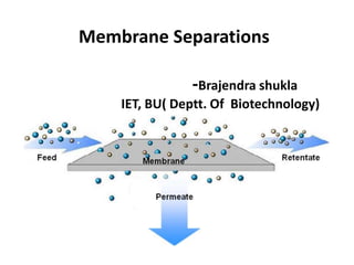
  • 1. Membrane Separations -Brajendra shukla IET, BU( Deptt. Of Biotechnology)
  • 3. Membrane separations: Introduction • Membranes are semi-permeable barrier used for – Particle-liquid separation – Particle-solute separation – Solute-solvent separation – Solute-solute separation • Applications – Product concentration – Product sterilization – Solute fractionation – Solute removal from solutions (desalination, demineralization) – Purification – Clarification
  • 4. Factors utilized in membrane separations • Solute size • Electrostatic charge • Other non-covalent interactions • Diffusivity • Solute shape
  • 5. Transport of material through a membrane Diffusion driven separation Pressure driven separation (convective transport) Membrane module Retentate Permeate Membrane Membrane module Retentate Permeate Membrane Sweep Feed Feed
  • 7. Membrane materials • Organic polymers – Polysulfone (PS) – Polyethersulfone (PES) – Cellulose acetate (CA) – Regenerated cellulose – Polyamides (PA) – Polyvinylidedefluoride (PVDF) – Polyacrylonitrile (PAN) • Inorganic materials – Glass – Metals – Ceramics – Layers of chemicals – Pyrolyzed carbon
  • 8. Membrane preparation by casting • Precipitation from vapour phase – This is achieved by penetration of the precipitant through a polymeric film from the vapour phase, which is saturated with the solvent used. • Precipitation by evaporation – The polymer is dissolved in a mixture of more volatile and less volatile solvents. As the more volatile component evaporates, the polymer precipitates to form the membrane. • Immersion precipitation – This involves immersion of the cast film in a bath of non-solvent for coagulation of the membrane material. • Thermal precipitation – The polymer is precipitated from solution by a cooling step.
  • 9. Other membrane making procedures • Stretching: – Involves stretching a polymer film at normal or elevated temperature in order to produce pores of desired size. • Sintering: – Powdered material is sintered by compression with/without heating to give microporous membranes. • Slip casting: – Most inorganic membranes are prepared using this method. – The method involves coating repeated layers of uniform particles with decreasing sizes on porous support.
  • 10. Other membrane making procedures • Leaching: – Some inorganic membranes are prepared by leaching technique. – Isotropic glass membranes are prepared by a combination of phase separation and acid leaching. • Track etching: – A homogeneous polymer film is exposed to laser beams or beams of collimated charged particles. – This breaks specific chemical bonds in the polymer matrix. – The film is then placed in an etching bath to remove the damaged sections thus giving rise to monodisperse pores
  • 12. Porous membranes Isoporous membrane Microporous symmetric Microporous asymmetric
  • 13. Basic forms of membranes • Flat sheet membrane • Tubular membrane • Hollow fibre membrane
  • 14. Factors influencing the performance of a membrane • Mechanical strength – Tensile strength, bursting pressure • Chemical resistance – pH range, solvent compatibility • Permeability to different species – Pure water permeability, sieving coefficient • Average porosity and Pore size distribution • Sieving properties – Nominal molecular weight cut-off • Electrical properties – Membrane zeta potential
  • 15. Driving force in membrane separation • Transmembrane (hydrostatic) pressure (TMP) • Concentration or electrochemical gradient • Osmotic pressure • Electrical field • Partial pressure • pH gradient
  • 16. Membrane processes that separate primarily based on size (pressure driven) 1 to 50 psi 10 to 100 psi 200 to 600 psi
  • 17. Membrane processes that separate based on principles other than size • Pervaporation – Separates a volatile or low-boiling-point liquid from a non-volatile liquid – The driving force is a vacuum on the gaseous side of the membrane – Tool for separation of liquid mixtures, especially dehydration of liquid hydrocarbons
  • 18. Applications of pervaporation • Dehydration of ethanol–water azeotrope • Removal of water from organic solvents • Removal of organics from water
  • 19. Membrane processes that separate based on principles other than size • Electrodialysis (ED) • Electrochemical process used to separate charged particles from an aqueous solution or from other neutral solutes • A stack of membranes is used, half of them passing positively charged particles and rejecting negatively charged ones; the other half doing the opposite. • An electrical potential is imposed across the membranes and a solution with charged particles is pumped through the system. • Positively charged particles migrate toward the negative electrode, but are stopped by a positive-particle-rejecting membrane • Negatively charged particles migrate in the opposite direction with similar results
  • 21. Flux • Throughput of material through a membrane • Flux depends on – Applied driving force – Resistance offered by membrane • Fouling – Increase in membrane resistance during a process – The decline in flux through a membrane with time in a constant force membrane process is due to fouling Flux Time Decline in flux due to fouling in a constant driving force membrane separation Pressure Time Fouling in constant flux membrane separation
  • 23. Membrane element and module Membrane element refers to the basic form of the membrane: • Flat sheet • Hollow fibre • Tubular Membrane module refers to the device which houses the membrane element: • Stirred cell module • Flat sheet tangential flow (TF) module • Tubular membrane module • Spiral wound membrane module • Hollow fibre membrane module
  • 24. Membrane modules Stirred cell unit Arrangement flat sheet TF module Small scale flat sheet TF module Pilot plant scale flat sheet TF module
  • 25. Stirred cell Membrane Stirrer bar Permeate/filtrate Nitrogen/compressed air Magnetic stirrer Feed Pressure gauge Permeate collection chamber •Research and small-scale manufacturing •Used for microfiltration and ultrafiltration •Excellently suited for process development work
  • 26. Flat sheet tangential flow module Feed Retentate Permeate Permeate Membranes •Similar plate and frame filter press •Alternate layers of membranes, support screens and distribution chambers •Used for microfiltration and ultrafiltration
  • 27. Spiral flow membrane module •Flat sheet membranes are fused to form an envelop •Membrane envelop is spirally wound along with a feed spacer •Filtrate is collected within the envelope and piped out
  • 29.
  • 31. Tubular membrane module Feed Retentate Permeate (flows radially) •Cylindrical geometry; wall acts as the membrane •Tubes are generally greater than 3 mm in diameter •Shell and tube type arrangement is preferred •Flow behaviour is easy to characterise
  • 32. Tubular membranes are used for all types of pressure driven separations Tubular modules are widely used where it is advantageous to have a turbulent flow regime Advantages 1. Low fouling and hence relatively easy cleaning 2. Easy handling of suspended solids & viscous fluids 3. Ability to replace or plug a damaged membrane. Disadvantages 1. High capital cost 2. Low packing density 3. High pumping costs 4. High dead volume Tubular membrane module
  • 33. Section of tubular module Large scale tubular module
  • 34. Hollow fibre membrane module •Similar to tubular membrane module •Tubes or fibres are 0.25 - 2.5 mm in diameter •Fibres are prepared by spinning and are potted within the module •Straight through or U configuration possible •Typically several fibres per module
  • 36. Plate and frame Spiral wound Tubular Hollow fiber Packing density 30 – 500 200 – 800 30 – 200 500 – 9000 Resistance to fouling Good Moderate Very good Poor Ease of cleaning Good Fair Excellent Poor Relative cost High Low High Low Main Applications D, RO, PV, UF, MF D, RO, GP, UF, MF RO, UF D, RO, GP, UF Comparison of different membrane modules
  • 37. Type Fluid flow regime Membrane area/module volume Mass transfer coefficient Hold-up volume Special remarks TF flat sheet Laminar- turbulent Low Low to moderate Moderate Can be dismantled and cleaned easily Spiral wound Laminar Moderate Low Low High pressures cannot be used Hollow fibre Laminar- turbulent High Low to moderate Low Susceptible to fibre blocking Tubular Turbulent Low Moderate to high Moderate to high Flow easy to characterize Excellently suited for basic membrane studies. Operating characteristics of membrane modules
  • 39. Membrane characterization The performance of a membrane process depends on the properties of the membrane: • Mechanical strength • Tensile strength, bursting pressure • Chemical resistance • pH range, compatibility with solvents • Permeability to different species • Pure water permeability, gas permeability • Average porosity and pore size distribution • Sieving properties • Nominal molecular weight cut-off • Electrical properties • Membrane zeta potential
  • 40. Ultrafiltration General Industrial Uses: Concentration of macromolecules Purification of solvent by removal of solutes Fractionation of macromolecules Clarification Retention of catalysts Analysis of complex solutions for specific solutes Bioprocess Applications: Fractionation of biological macromolecules e.g. proteins, DNA Concentration of polymer solutions Removal of LMW solutes from protein solutions Removal of cells and cell debris from fermentation broth Virus removal from therapeutic products Harvesting of biomass e.g., cells and sub-cellular products Membrane bioreactors Effluent treatment
  • 41. Ultrafiltration membranes •Pores: 10 to 1000 Angstroms •Generally anisotropic (skin layer 0.2 to 10 micron thick) •Properties of an ideal ultrafiltration membrane: •High hydraulic permeability to solvent •Sharp “retention cut-off” properties: The membrane must be capable of retaining completely nearly all the solutes above some specified value, known as the molecular cut-off (MWCO) •Good mechanical durability •Good chemical and thermal stability •Excellent manufacturing reproducibility and ease of manufacture
  • 42. Sharp and diffuse cut-off membranes
  • 43. Ultrafiltration: Pore flow model p p m v l P d J   32 2   Jv = Permeate flux m =Membrane porosity dp = Average pore diameter P =Transmembrane pressure  =Viscosity Lp =Average pore length f o i P P P P - +   2 Membrane Retentate Feed Permeate/filtrate Pi Po Pf Hagen-Poiseuille’s law for permeate flux of pure solvent Pi and Po inlet and outlet pressures on the feed side Pf is the pressure on the filtrate side The pressure drop for a Cross flow membrane module
  • 44. Ultrafiltration: Flux equations Pore flow model: UF of solvent p p m v l P d J   32 2   Resistance model: UF of solvent m v R P J   Osmotic pressure model: UF of solution cp m v R R P J +  -    g cp m v R R R P J + +  -    Rm = membrane hydraulic resistance Rcp = resistance due to concentration polarization Rg = gel layer resistance Rm = membrane hydraulic resistance
  • 45. Concentration polarization Membrane Bulk feed db = Thickness ofconcentration polarization layer Cb Cw Cp Permeate
  • 46. Concentration polarization model UF of solution         - -  p b p w v C C C C k J ln 0 v v p dC J C J C D dx - +  Material balance in a control volume within the concentration polarization layer at steady state Upon integration with boundary conditions C= Cw at x=0 and C=Cb at x=δb we get concentration polarization equation for partially rejected solutes For total solute rejection i.e, Cp = 0 ln w v b C J k C        When Cw is equal to the gelation concentration, there will be no further increase in the value of Cw Hence we write gel polarization equation as lim ln g b C J k C       
  • 47. Effect of transmembrane pressure on permeate flux Permeate flux Transmembrane pressure Pressure dependent Pressure independent ? Limiting flux At constant TMP the permeate flux decreases as the feed concentration increases When Cw = Cg the permeate flux is independent of the TMP
  • 48. Problem A protein solution (conc, 4.4 g/l) is being ultrafiltered using a spiral wound membrane module which totally retains the protein. At a certain transmembrane pressure the permeate flux is 1.3x10⁻⁵ m/s. The diffusivity of the protein is 9.5 x 10⁻¹¹ m2/s while the wall concentration at this operating pressure is estimated to be 10 g/l. Predict the thickness of the boundary layer. If the permeate flux is increased to 2.6 x 10⁻⁵ m/s while maintaining the same hydrodynamic conditions within the membrane module, what is the new wall concentration?
  • 49. Where there is total retention we can use the equation This equation can be written as The mass transfer coefficient is given by Therefore When Jv is increased to 2.6 x 10⁻⁵ m/s and k remains the same, the wall concentration can be obtained from the concentration polarization equation for totally retained solute ln w v b C J k C        5 5 1.3 10 1.584 10 / 10 ln ln 4.4 v w b J k m s C C - -                  b D k d  11 6 5 9.5 10 5.99 10 1.584 10 b m m d - - -      6 5 2.6 10 exp 4.4 exp / 22.727 / 1.584 10 w b Jv C C g l g l k - -                  
  • 50. Effect of feed concentration on permeate flux TMP Jv Cb Jlim ln Cb Cs or Cg k For a given feed concentration, the limiting flux increases with increases in mass transfer coefficient Permeate flux decreases as the feed concentration is increased
  • 51. Mass transfer coefficient (k) Affects back-diffusion of accumulated solute Measure of the hydrodynamic conditions within the module k = (D/db) Mass transfer coefficient can be measured experimentally •Plot of limiting flux versus log of feed concentration •Plot of sieving parameter versus (Jv/k) Mass transfer coefficient can be estimated using heat-mass transfer analogy •Dimensionless equations: Sherwood number as function of Reynolds number and Schmidt number
  • 52. Schmidt number = Momentum transfer/Mass transfer kd Sh D        Reynolds number = Inertial forces/Viscous forces Sherwood number = Total mass transfer/Diffusive mass transfer Re du du                 v Sc D D                 Mass transfer correlations Peclet number = Convective mass transfer / Diffusive mass transfer h d Pe D  Grashof number = Gravitational forces/ Viscous forces 3 2 2 ' L B g t Gr     Froude number = Interial forces/ Gravitational forces 2 v Fr gL 
  • 53. Mass transfer correlations Fully developed laminar flow (i.e. Re < 1000) in tubular membrane 0.33 0.33 0.33 1.62 Re t d Sh Sc l        Turbulent flow (i.e. Re > 2000) in tubular membrane 33 . 0 8 . 0 Re 023 . 0 Sc Sh  Graetz-Leveque Dittus-Boelter Fully developed laminar flow 33 . 0 67 . 0 33 . 0 816 . 0 -  t L D k  Porter Shear rate at the wall  = 8 ul / d for tubes  = 6 ul / b for rectangular channels (b = channel depth)
  • 54. Problem: Shear-Induced Diffusivity Shear-induced diffusivity is 3 x 10⁻⁷ cm2/s. Hydrodynamic diffusivity is 2 x10⁻⁹ cm2/s. Shear-induced diffusivity is about 150 times larger. 6 A A RT D R N   2 s w D a   Compare hydrodynamic and shear-induced diffusivity values for a 1-mm particle at a shear rate of 1,000 s-1. Assume the value of α to be 0.03 for ultra filtration processes
  • 55. 0.8 0.33 0.023 Re Sh Sc  Problem: Calculate the mass transfer coefficient for ultrafiltration of milk at 50oC employing tubular membrane system with the following configurations: Pore diameter of 1.25 cm; Length = 240 cm; Number of channels = 18; superficial velocity = 200 cm/sec; Pressure drop over length = 2 kg/cm2. The physical properties of milk are as follows: Density = 1.03 g/ml; viscosity 0.008 g/cm/sec; Diffusivity = 7.0 x 10⁻⁷ cm2/sec. The bulk protein concentration is 3.1% and the gel protein concentration is 22%. Assume turbulent regime for the process and make use of Dittus-Boelter correlation
  • 56. 3 1.25( ) 200( / sec) 1.03( / ) Re 0.008( / / sec) du du cm cm g cm g cm                     = 32188 3 7 2 0.008( / / sec) 1.03( / ) 7 10 ( / sec) v g cm Sc D D g cm cm   -                  = 11096 For calculating Sherwood number in turbulent flow regime (i.e. Re > 2000) in tubular membrane, Dittus-Boelter correlation can be used 0.8 0.33 0.8 0.33 0.023 Re 0.023 (32188) (11096) Sh Sc     = 2008
  • 57. kd Sh D        Now for calculating mass transfer coefficient k we will make use of the Sherwood number 7 2 2 2 2 2008 7 10 ( / sec) 1.25( ) 0.0011( / / sec) 60 10 ( / / ) DSh cm k d cm cm cm litre m hr - -        To calculate the flux for the process 2 2 22 ln 60 10 ln 79.3654 / / 3.1 g b C J k litre m hr C -                
  • 58. Calculate the mass transfer coefficient for ultrafiltration of milk at 50oC employing tubular membrane system with the following configurations: Pore diameter of 1.25 mm; Length = 240 cm; Number of channels = 18; superficial velocity = 200 cm/sec; Pressure drop over length of tube = 2 kg/cm2 Shear rate at wall = 7272.0 /sec The physical properties of milk are as follows: Density = 1.03 g/ml; viscosity 0.008 g/cm/sec; Diffusivity = 7.0 x 10⁻⁷ cm2/sec. The bulk protein concentration is 3.1% and the gel protein concentration is 22%. Assume turbulent regime for the process and make use of Dittus-Boelter correlation
  • 59. Effect of hydrodynamic parameters on permeate flux Crossflow velocity Permeate flux Mass transfer coefficient Reynolds number Turbulent Laminar
  • 60. Enhancement of permeate flux • By increasing the cross-flow rate • By creating pulsatile flow • By pressure pulsing • By creating oscillatory flow • By flow obstruction using baffles • By generating Dean vortices • By generating Taylor vortex • By gas-sparging into the feed
  • 61. Dean vortices • Dean vortices are helicoidal flows created by centrifugal forces in curved channels – Coiled or helically twisted tubular membranes • Enhance solute back transfer away from the membrane • Effective for enhancing permeate flux by depolarization of the solute layer on the membrane
  • 62. Dean vortices • Dean vortices are secondary tangential flows that create a self-cleaning flow mechanism when induced within a cross- flow filtering system • The general principle of this technology – to design, develop and use these tangential flows to sweep around a curve to “clean” the membrane, leading to enhanced filter performance and longer membrane life
  • 63. Taylor Vortex • Specialised type of Couette flow • When the angular velocity of the inner cylinder is increased above a certain threshold • Couette flow becomes unstable and a secondary steady state characterized by axisymmetric toroidal vortices Plasma collection from donors in transfusion centers by microfiltration
  • 64. Plasma cell filter for plasma collection from donors with a rotating cylindrical membrane DYNAMIC FILTRATION Biodruckfilter (sulzer AG, Winterthur, Switzerland) http://www.sulzer.com. Rotary biofiltration device (Membrex Inc.) and merged into GE Osmonic (www.gewater.com)
  • 65. Rotating Disk Modules MSD system (Westfalia Separator, Aalen, Germany) Multishaft systems with overlapping rotating membranes The MSD system features 31-cm- diameter ceramic membranes on eight parallel shafts located on a cylinder for a membrane area of 80 m2 All disks rotate at the same speed and are enclosed in a cylindrical housing The membrane shear rate is unsteady and reaches a maximum in the overlapping regions
  • 66. Rotating disk dynamic filtration system (Pall Corp., Massachusetts, USA) www.pall.com Dyno (Bokela GmbH, Karlsruhe, Germany) www.bokela.com Optifilter CR (Metso Paper, Raisio, Finland) www.metso.com/ Multi-disk system (SpinTek, Huntington, CA, USA) www.spintek.com MSD system (Westfalia Separator, Aalen, Germany) www.westfalia- separator.com Rotostream (Canzler, Dueren, Germany) http://www.sms-vt.com/index.php Multishaft disk (MSD) system (Hitachi Ltd.) www.hitachi.com Self Cleaning Filtration, (novoflow, Oberndorf, Germany) http://www.novoflow.com/en/home Rotating Disk Modules
  • 67. Flux Enhancement by Pulsatile Flows • Another method for enhancing permeate flux and mass transfer without using very high fluid velocity • Consists of superposing flow and pressure pulsations at the membrane inlet with a piston-in-cylinder system or special pumps such as modified roller pumps Pulsatile blood flow to enhance gas transfer in membrane blood oxygenators
  • 68. Retrofiltration • Technique for reducing membrane fouling by pressurizing the permeate above retentate pressure in order to inject permeate into retentate and clean the pores – Backwashing – Backpulsing
  • 69. Vibratory shear-enhanced processing Schematic of the vibratory shear-enhanced processor (VSEP) pilot series L with a single membrane oscillating around its vertical axis Vibratory shear-enhance processing (VSEP) (New Logic Research, Inc.) www.vsep.com PallSep Vibrating Membrane Filter (Pall Corporation) http://www.pall.com
  • 70. Solute transmission through UF membranes Amount of solute going through an UF membrane can be quantified in terms of the membrane intrinsic rejection coefficient (Ri) or intrinsic sieving coefficient (Si): i w p i S C C R -  -  1 1 Cw is difficult to determine and hence it is more practical to use the apparent rejection coefficient (Ra) or the apparent sieving coefficient (Sa): a b p a S C C R -  -  1 1
  • 71. Factors influencing the retention of a solute by membrane • Primary variable – Solute diameter to pore diameter ratio • Also depends on – Solute shape – Solute charge – Solute compressibility – Solute-membrane interactions – Operating conditions The amount of solute going through the membrane can be quantified in terms of intrinsic rejection coefficient (Ri) and intrinsic sieving coefficient (Si)
  • 72. Rejection coefficient: Older theory  new theory    2 2   -  a R 1  a R for  < 1 for   1  = (di / dp)=solute-pore diameter ratio In other words, Ra is constant for a solute- membrane system. It is now recognised that rejection coefficients depend on operating and environmental parameters such as •pH •Ionic strength •System hydrodynamics •Permeate flux  1 p i w C R C  - 1 p a b C R C  -
  • 73. Sieving coefficients w p i C C S  Intrinsic sieving coefficient •Depends on solute-membrane system •Depends on physicochemical parameters such as pH and ionic strength •Depends on permeate flux Apparent sieving coefficient •Depends on solute-membrane system •Depends on physicochemical parameters such as pH and ionic strength •Depends on permeate flux •Depends on system hydrodynamics b p a C C S 
  • 74. Effect of permeate flux on intrinsic sieving coefficient 1 exp exp -         +              eff m v eff m v i D J S S D J S S S d d Intrinsic sieving coefficient Permeate flux (log scale) Asymptotic intrinsic sieving coefficient S͚
  • 75. Effect of permeate flux and mass transfer coefficient on apparent sieving coefficient           + +                 - -         +        k J D J S S D J S S k J D J S S S v eff m v eff m v v eff m v a d d d exp exp 1 1 exp Permeate flux (log scale) Apparent sieving coefficient Mass transfer coefficient Apparent sieving coefficient
  • 76. Determination of intrinsic sieving coefficient and mass transfer coefficient       +         -          - k J S S S S v i i a a 1 ln 1 ln         - a a S S 1 ln       k Jv         - i i S S 1 ln
  • 77. Problem The intrinsic and apparent rejection coefficients for a solute in an ultrafiltration process were found to be 0.95 and 0.63 respectively at a permeate flux value of 6 x 10⁻³ cm/s. What is the solute mass transfer coefficient?
  • 78. Solution:       +         -          - k J S S S S v i i a a 1 ln 1 ln Sa = 1-Ra = 1-0.63 = 0.37 Si = 1-Ri = 1-0.95 = 0.05 ln ln 1 1 v a i a i J k S S S S      -     - -     3 3 6 10 / 0.37 0.05 ln ln 1 0.37 1 0.05 2.486 10 / k cm s cm s - -       -     - -      
  • 79. Solute fractionation For fractionation of a binary mixture of solutes, it is desirable to achieve maximum transmission of the solute desirable in the permeate and minimum transmission of the solute desirable in the retentate.     2 1 2 1 1 1 a a a a R R S S - -    Enhancement of fractionation • pH optimization • Feed concentration optimization • Salt concentration optimization • Membrane surface pre-treatment • Optimization of permeate flux and system hydrodynamics Selectivity parameter
  • 80. Problem A feed solution (10 g/l) of dextran (MW=505 kDa) is ultrafiltered through a 25 kDa MWCO Membrane. The pure water flux values and the dextran UF permeate flux values at different TMP are given below The osmotic pressure is given by the following correlation where Δπ is in dynes/cm2 and Cw is in %w/v. Calculate the membrane resistance and the mass transfer coefficient for dextran assuming that Rg and Rcp are negligible ΔP (kPa) Pure water flux (m/s) Jv (m/s) 30 9.71x10⁻⁶ 6.24x10⁻⁶ 40 1.23 x 10⁻⁵ 7.08x10⁻⁶ 50 1.57x10⁻⁵ 7.63x10⁻⁶ 60 1.87x10⁻⁵ 8.02x10⁻⁶ 0.35 log 2.48 1.22( ) w C    +
  • 81. y = 3E-07x + 4E-07 0.00E+00 2.00E-06 4.00E-06 6.00E-06 8.00E-06 1.00E-05 1.20E-05 1.40E-05 1.60E-05 1.80E-05 2.00E-05 0 20 40 60 80 Plot of Pure water flux vs transmembrane pressure Pure water flux (m/s) Linear (Pure water flux (m/s) ) Solution The MWCO of the membrane is 25 kDa while the MW of dextran is 505 kDa. Hence we can safely assume that dextran is totally retained. Pure water ultrafiltration is governed by m v R P J   Rm = 3.33 x 10⁹ Pa.s/m
  • 82. v m cp g P J R R R   -   + + We also know that v m P J R   -   Since Rcp and Rg are negligible the equation becomes Using the above equation we can calculate the osmotic pressure for every value of transmembrane pressure ΔP (kPa) Pure water flux (m/s) Jv (m/s) Δπ (kPa) Δπ (dynes/c m2) Cw (%w/v) Cw (g/l) K (m/s) 30 9.71x10⁻⁶ 6.24x10⁻⁶ 9.22 92208 7.63 76.31 3.07x10⁻⁶ 40 1.23 x 10⁻⁵ 7.08x10⁻⁶ 16.42 164236 10.04 100.43 3.7x10⁻⁶ 50 1.57x10⁻⁵ 7.63x10⁻⁶ 24.59 245921 11.99 119.94 3.07x10⁻⁶ 60 1.87x10⁻⁵ 8.02x10⁻⁶ 33.29 332934 13.61 136.08 3.07x10⁻⁶
  • 83. The correlation for osmotic pressure given in the problem can be rearranged to   2.857 log10 2.48 1.22 w C   -        Using the above equation the wall concentration at different TMP can be calculated The mass transfer coefficient in an UF process with total solute retention is given by ln w v b C J k C        Rearranging the equation we get ln v w b J k C C       
  • 84. Microfiltration • Microfiltration separates micron-sized particles from fluids • The modules used for microfiltration are similar to those used in ultrafiltration • Microfiltration membranes are microporous and retain particles by a purely sieving mechanism Microfiltration can be operated either in dead-ended (normal flow) mode or cross- flow mode Typical permeate flux values are higher than ultrafiltration processes even though the processes are operated at much lower TMP
  • 85. Applications of microfiltration • Cell harvesting from bioreactors • Virus removal for solutions • Clarification of fruit juice and beverages • Removal of cells from fermentation media • Water purification • Air filtration • Sterilization
  • 86. The permeate flux in microfiltration ) ( C M v R R P J +    Jv = Permeate flux P = Pressure difference across the membrane RM = Membrane resistance RC = Cake resistance  = Liquid medium viscosity The cake resistance M S C A V r R  r = Specific cake resistance VS = Volume of cake AM = Area of membrane For micron sized particles, r is given by               -  2 3 1 1 180 s d r    = Porosity of cake ds = Mean particle diameter
  • 87. Problem: Microfiltration of bacteria Bacterial cells having 0.8 micron average diameter are being microfiltered in the cross-flow mode using a membrane having an area of 100 cm2. The steady state cake layer formed on the membrane has a thickness of 10 microns and a porosity value of 0.35. If the viscosity of the filtrate obtained is 1.4 cP, predict the volumetric premeate flux at a transmembrane pressure of 50 kPa. When pure water of viscosity 1 cP was filtered through the same transmembrane pressure, the permeate flux obtained was 10-4 m/s
  • 88. v M P J R    For pure water filtration the flux is written as 11 3 4 50000 5 10 / (1 10 ) (1 10 ) M v P R m J  - - -         The specific cake resistance of the bacterial cell cake can be calculated from The cake resistance Rc can be calculated from 15 2 3 2 3 7 2 1 1 1 0.35 1 180 180 4.264 10 / 0.35 (8 10 ) s r m d   -     - -                         15 5 10 4.264 10 1 10 4.264 10 / S C c M V R r r m A d -         Solution
  • 89. The permeate flux can be calculated from 3 10 11 50000 ( ) 1.4 10 (4.264 10 5 10 ) v M C P J R R  -    +    +  = 6.58 x 10⁻⁵ m/s
  • 90. Dialysis • The mode of transport in dialysis is diffusion • Separation occurs because – Small molecules diffuse more rapidly than larger ones – Also due to the degree to which the membrane restricts transport of molecules usually increases with solute size Membrane Bulk concentration on downstream side (C2) Boundary layers Concentration profile in dialysis Bulk concentration on upstream side (C1)
  • 91. The rate of mass transport or solute flux (N) is directly proportional to the difference in concentration (C) at the membrane surfaces d C SD N eff   S is a dimensionless solute partition coefficient Deff is the effective diffusivity of the solute within the membrane d is the membrane thickness Deff and d can be combined and termed the membrane mass transfer coefficient (KM) for a given membrane-solute system M M R C C K N     Dialysis
  • 92. 2 1 1 1 1 1 K K K K M O + +  KO = the overall mass transfer coefficient K1 and K2 are the mass transfer coefficients on the upstream and downstream sides   2 1 C C K N O -  In terms of mass transfer coefficient C1 and C2 are the upstream (feed) and downstream (dialysate) concentrations 2 1 R R R R M O + +  The membrane resistance alone seldom governs the overall mass transport. The liquid boundary layers on either side of the membrane also contribute to resistance to transport RO = the overall resistance R1 = the resistance on the upstream surface R2 = the resistance on the downstream surface
  • 93. Hollow fiber dialyser C1 C2 C3 C4 Co-current flow Counter-current flow C1 C3 C2 C4 Feed Dialyzing solution (sweep stream) Dialysate Product Feed Dialyzing solution (sweep stream) Dialysate Product
  • 94. Co-current and counter-current dialysis         - - - - -   4 2 3 1 4 2 3 1 ln ) ( ) ( C C C C C C C C Clm Log-mean concentration difference (∆Clm) Co-current Counter-current         - - - - -   3 2 4 1 3 2 4 1 ln ) ( ) ( C C C C C C C C Clm Length of membrane Conc. Feed side Dialysate Conc. Length of membrane Feed side Dialysate
  • 95.         - - - - -   4 2 3 1 4 2 3 1 ln ) ( ) ( C C C C C C C C Clm Co-current flow Co-current operation is preferred when liquid flow causes significant pressure drop between inlet and outlet side Generally in co-current mode membrane utilization is incomplete
  • 96.         - - - - -   3 2 4 1 3 2 4 1 ln ) ( ) ( C C C C C C C C Clm Counter-current flow Counter current mode ensures uniform gradient and hence uniform solute flux Counter current dialysis is most commonly used as it ensures full membrane utilization
  • 97. Co-current flow Counter-current flow C1 C3 C3 C4 C1         - - - - -   4 2 3 1 4 2 3 1 ln ) ( ) ( C C C C C C C C Clm         - - - - -   3 2 4 1 3 2 4 1 ln ) ( ) ( C C C C C C C C Clm Dialysis modes C4
  • 98. Applications of dialysis • Removal of acid or alkali from products • Removal of alcohol from beer (to make alcohol free beer) • Removal of salts and low molecular weight compounds from solutions of macromolecules • Concentration of macromolecules • Dialysis provides a tool for controlling the chemical species within a reactor • Purification of biotechnological products • Haemodialysis
  • 99. The figure below shows a completely mixed dialyser unit. Plasma having a glutamine concentration of 2 kg/m3 is pumped into the dialyser at a rate of 5x10⁻⁶ m3/s and water at a flow rate of 9 x 10⁻⁶ m3/s is used as the dialysing fluid. If the membrane mass transfer coefficient is 2 x 10⁻⁴ m/s and the membrane area is 0.05 m2, calculate the steady state concentrations of glutamine in the product and dialysate streams. Problem
  • 100. Solution The overall material balance for glutamine gives ------- (a) The glutamine concentration flux per unit area can be obtained using equation The amount of glutamine in of the dialysate should be equal to the product of the concentration flux and area: The amount of glutamine in the dialysate = Q2C4, therefore ------- (b) Solving the two equations simultaneously, we get: C2 = 1.027 kg/m3 C4 = 0.541 kg/m3 2 4 ( ) c m m J K C K C C    - 2 4 * * * ( ) c m m J A K A C K A C C    - 2 4 2 4 Q C K *A(C C ) m  - 1 1 l 2 2 4 Q C Q C Q C  +
  • 101. Packed bed adsorption has several major limitations • High pressure drop • Increase in pressure drop during operation • Column blinding by proteins • Dependence on intraparticle diffusion for the transport of proteins to their binding sites • High process times (due to iv) • High flow rates cannot be used • High recovery liquid volume • Radial and axial dispersion resulting from the use of polydisperse media • Problems associated with scale-up
  • 102. Advantages of membrane adsorbers • Low process time • Low recovery liquid volume • Possibility of using higher flow rates • Lower pressure drop • Less column blinding • Ease of scale-up • Fewer problems associated with validation (if a disposable membrane is used)
  • 103. Comparison of solute transport in particulate packed bed and membrane adsorbers
  • 104.
  • 105. Different types separation chemistries are used in membrane adsorption • Affinity binding • Ion-exchange interaction • Reverse phase and hydrophobic interaction Size exclusion based separation using membrane beds has not yet been feasible
  • 106. Membrane adsorption • Membrane adsorption processes are carried out in two different modes – Pulse – Step • Based on the membrane geometry, three types of membrane adsorbers are used: – Flat sheet – Radial flow – Hollow fibre
  • 107. Operation of flat sheet membrane adsorber
  • 108. Operation of hollow fibre membrane adsorber
  • 109. δm θC θD Diffusion and convection times in membrane adsorption Re s pore pore u d v        Reynolds number of the fluid flowing through the membrane pores us = superficial velocity (m/s) dpore = average pore diameter (m) v = kinematic viscosity (m2/s) ε = porosity (-) 2 m c s u d    2 4 pore d d D   Time taken for solute to diffuse from central line to the pore wall Residence time of solute moving along central line through a pore dpore
  • 110. An adsorptive membrane has a thickness of 2 mm and a diameter of 5 cm. The porosity of the membrane is 0.75 and the tortuosity is 1.5. The pore diameter was estimated to be 2 x 10⁻⁶ m. If we are to use this membrane for adsorption of a DNA fragment (diffusivity = 9.5 x 10⁻¹² m2/s) from an aqueous solution, what is the maximum solution flow rate that can be used? Assume that the flow through the pores is laminar Problem: Membrane adsorption of DNA
  • 111. Area of the membrane = 1.964 x 10⁻³ m2 The superficial velocity is given by The convection time can be obtained from Diffusion time can be calculated using For total capture of DNA θC > θD . Therefore The solution flow rate should be lower than 2.098 x 10⁻⁵ m3/s. 3 3 2 ( / ) / 1.964 10 ( ) s Q Q m s u m s A m -    3 3 6 2 10 ( ) 1.5 0.75 1.964 10 2.2095 10 2 2 m c s m s u Q Q d   - - -          2 6 2 12 (2 10 ) 0.1053 4 4 9.5 10 pore d d s D  - -       6 2.2095 x10 0.1053 Q -  Solution
  • 112. ChromaSorb™ Membrane Adsorber (Millipore) Single-use, flow-through anion exchanger designed for the removal of trace impurities including host cell protein (HCP), DNA, endotoxins and viruses from monoclonal antibody or other protein feedstocks.
  • 114. Schematic representation of membrane adsorber and the operations of one purification cycle
  • 115. Liquid membrane technology • Liquid membrane extraction involves – the transport of solutes across thin layers of liquid interposed between two otherwise miscible liquids • There are two types of liquid membrane processes: – Emulsion liquid membrane (ELM) processes – Supported liquid membrane (SLM) processes
  • 118. Schematic diagram of the membrane emulsification process
  • 119. Limitations 1. Film diffusion 2. Pore diffusion 3. Binding kinetics Limitations 1. Film diffusion 3. Binding kinetics
  • 121. Introduction • In RO, the goal is usually to remove a solute from solution by passing the solvent through the membrane and leaving the solute in a concentrated retentate (reject) stream • Note that this is a continuous process, unlike filtration; purified water is produced continuously
  • 122. Advantages • low energy consumption • high removal of solute in one stage • no components added (such as absorbing gas or extracting liquid) • no phase change • low capital costs • easy, modular, installation
  • 123. Disadvantages • Membrane life (hopefully 3-5 years) • Fouling • Pretreatment costs (removal of suspended solids, fouling materials) • Relatively low concentration of solutes • In order to understand and to predict membrane performance it is necessary to have transport equations that describe the transport of solvent and solute through the membrane • In all membrane processes, we are looking at relationships between forces (driving forces) and fluxes; – [Class: you name some examples of these relationships that you already know.]
  • 124. Osmotic Pressure • Thermodynamic property of a solution which represents how different a solution is compared to a pure solvent in terms of the pressure required to bring the solution up to the same chemical potential (ie., in equilibrium with) pure solvent – what this means, practically, is that osmotic pressure acts against the pressure driving force for transport across a membrane. • This osmotic pressure can be 'looked up' in a book - a thermodynamic property. • A reasonable approximation of osmotic pressure is the Van't Hoff Eqn where n is the kmol of solute per Vm m3 of pure solvent, which is the same as the molar concentration, ci
  • 125. Osmotic pressure cRT   2 3 1 2 3 ( ......) RT AC A C A C   + + + For concentrated solutions of uncharged solutes correlations involving series of virial coefficients are used van’t Hoff equation The osmotic pressure difference across a membrane is given by 1 2     -
  • 126.
  • 127. Summary of the transport equations Solvent flux ) (   -   P A N W W ) ( P A N W W   Pure water flux Solute Flux ) ( ) ( 2 2 c c A c c L K D N b S b M S S S -  -  Concentration Polarization ) ( ) ( ln 2 1 2 c c c c k c N N c N J b S W T V - -  +   Material Balance on Solute S W S N N N c c +  2