Design of Rigid frame using Midas Gen

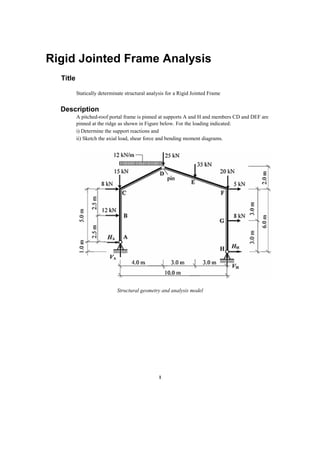
1. 1
Rigid Jointed Frame Analysis
Title
Statically determinate structural analysis for a Rigid Jointed Frame
Description
A pitched-roof portal frame is pinned at supports A and H and members CD and DEF are
pinned at the ridge as shown in Figure below. For the loading indicated:
i) Determine the support reactions and
ii) Sketch the axial load, shear force and bending moment diagrams.
Structural geometry and analysis model

2. 2
Finite Element Modelling:
 Analysis Type: 2-D static analysis (X-Z plane)
Step 1: Go to File>New Project and then go to File>Save to save the project with any name
Step 2: Go to Model>Structure Type to set the analysis mode to 2D (X-Z plane)
 Unit System: kN,m
Step 3: Go to Tools>Unit System and change the units to kN and m.

3. 3
 Geometry generation:
Step 4: Go to Model>Nodes>Create Nodes and type in (0,0,0) in the Coordinates box. Press
Apply. Switch to the Front view by clicking on as shown below. Switch on node number
from the option . Node number 1 will be point A.
Step 5: Go to Model>Element>Extrude Elements. Select type as Node->Line. Use select
single button to highlight the node number 1 by clicking on it. Type in (0,0,2.5) in the
Equal Distances dx,dy,dz box and enter number of times=2 and click Apply to generate the
column.

4. 4
Step 6: Similar to Step 5, select this time node number 3 and enter dx,dy,dz as (4,0,2) m,
number of times=1 and click Apply to generate the pitched roof.

5. 5
Step 7: Select node 4 and extrude using dx,dy,dz= (3,0,-1) and number of times = 2 and
Apply to generate the other half of the pitched roof.
Step 8: Finally Select node 6 and extrude using dx,dy,dz= (0,0,-3) and number of times=2
and click Apply and Close to generate the other column.

6. 6
 Material: Modulus of elasticity, E = 2.0 × 108
kN/m2
Step 9: Go to Properties>Material Properties>Add. Select User defined in the Type of
Design and Enter E=2.0 × 108
kN/m2
. Enter a name for the material and click OK and Close.
 Section Property: BS Column section UC 305x305x158
Step 10: Go to Properties>Section Properties>Add. Select DB/User tab and select I
section type. Select BS4-93 from section DB and select the section UC 305x305x158 from
the dropdown. Click OK and Close.
You can see the shape of the section in the model generated. Go to the Works Tree to check
the information for your model.

7. 7
 Boundary Condition: Pinned Supports at A and H and a pinned connection between
members CD and DEF at point D.
Step 11: Use select single to select or highlight nodes 1 and 8 as shown in figure below.
Go to Model>Boundaries>Supports and check on Dx and Dz and Apply.

8. 8
This becomes the Pinned support at A and H. DX and DZ provide horizontal and vertical
restraint simultaneously. No rotational restraint has been provided.
Step 12: Select and display element numbers by clicking on . Again use Select Single ,
this time to highlight or select element 3. Go to Model>Boundaries>Beam End Release.
Select Fixed-Pinned and Apply and Close.
This applies a moment release or a pinned connection at point D.
 Load Case:
Concentrated Loads:
-Vertically downward loads of 15 kN, 25 kN, 35 kN and 20 kN at points C, D, E and F
respectively applied in (-Z) direction.
-Horizontal Loads of 12kN, 8kN, 5kN and 8kN at points B, C, F and G respectively applied
in (+X) direction.
Step 13: Go to Load>Static Load Cases and define static load case ‘P’. Select Load type as
User defined for both of them. Click Close after adding the load case.

9. 9
Step 13: Go to Load>Nodal Loads and select load case P. Select the node 2 using and
enter FX=12 kN and press Apply. Select Node 3 and enter FX=8 kN and FZ = -15 kN and
Apply. Select Node 4 and enter FZ=-25 kN and Apply. Select Node 5 and enter FZ=-35 kN
and Apply. Select Node 6 and Apply FX=5 kN and FZ= -20 kN. Select node 7 and Apply
FX=8 kN.

10. 10
You can display the values from the Works Tree by Right clicking on Nodal Loads and click
Display.
Uniform Loads: A uniformly distributed load, UDL of 12 kN/m is applied vertically
downward on the member CD.
Step 14: Go to Loads>Element Beam Loads and select load case P. Select the element
number 3 and enter w=-12 kN/m in the Global Z direction and select Projection as Yes and
press Apply and Close.
From the display, the UDL looks as if it has been applied over the length of the element 3
but internally it has been applied only on the projected length i.e. X direction length of that
element since the Projection ‘Yes’ was selected while applying the load.
The analysis results for forces and moments in the frame are generated in the finite element
software with respect to each element’s local axis or centroidal axis. So before running the
analysis, we must make sure that the local axes of all elements are aligned properly. Turn on
the isometric view using . To display the local axis, go to View>Display and select
Element tab and check on Local axis and click OK. You will find that the members A to C
or the element numbers 1 and 2 have their local y axis inclined in the opposite direction to
the rest of the model’s y local axis. This may result in opposite signs for bending moments,
My.

11. 11
Check off node numbers and element numbers . Also display only wireframe by
clicking on for clarity.
Now to align the local axis properly, go to Model>Elements>Change Element
Parameters and go to Element Local Axis and select the 2 elements 1 and 2 that need to be
changed and enter the change in beta angle (local axis angle)=180 degrees in the Change
Mode.

12. 12
You can now undisplay the local axis by going back to View>Display and checking off
Local Axis in the Element tab and click Apply. Switch to front view by clicking on
from right.
 Analysis:
Step 15: Go to Analysis>Perform Analysis
Results
 Reaction Forces:
Step 16: Click on Results>Reactions>Reaction Forces/Moments and select the load case
P. Select FXYZ. Check on Values and click on the box next to Values to change number
of decimal points to 2 and click OK to see reactions graphically.

13. 13
 Beam forces/moment diagrams:
Step 17: Click on Results>Forces>Beam Diagrams and select the load Case P. Select Fx
and Click OK to display the axial force diagram in the members. Note that the ‘+’ sign
indicates Tension and ‘-‘ indicates Compression.

14. 14
Step 18: Change to Fz to view the shear force diagram and click Apply.

15. 15
Step 19: Change to My to calculate the Bending Moment Diagram.

16. 16
Hand Calculations:
(1) To determine support reactions
Taking vertical force sum:
𝚺𝑉 = 𝟎
𝑉𝐴 − 15.0 − (12.0 × 4.0) − 25.0 − 35.0 − 20.0 + 𝑉𝐻 = 0
𝑉𝐴 + V𝐻 = 143 Equation (1)
Taking horizontal force sum:
Σ𝐻 = 0
+𝐻𝐴 + 12 + 8.0 + 5.0 + 𝐻𝐻 = 0
𝐻𝐴 + 𝐻𝐻 = −25.0 𝐸𝑞𝑢𝑎𝑡𝑖𝑜𝑛 (2)
Taking sum of moments about A:
Σ𝑀𝐴 = 0
(12 × 2.5) + (8.0 × 5.0) + (12.0 × 4.0)(2.0) + (25.0 × 4.0) + (35.0 × 7.0)
+(20.0 × 10.0) + (5.0 × 5.0) + (8.0 × 2.0) − (𝐻𝐻 × 1.0) − (𝑉𝐻 × 10.0) = 0
𝐻𝐻 + 10.0𝑉𝐻 = 752 𝐸𝑞𝑢𝑎𝑡𝑖𝑜𝑛 (3)
Taking sum of moments about the Pin D:
Σ𝑀𝑝𝑖𝑛 = 0
+(35.0 × 3.0) + (20.0 × 6.0) − (5.0 × 2.0) − (8.0 × 5.0) − (𝐻𝐻 × 8.0) − (𝑉𝐻 × 6.0) = 0
8.0𝐻𝐻 + 6.0𝑉𝐻 = 175 𝐸𝑞𝑢𝑎𝑡𝑖𝑜𝑛 (4)

17. 17
From Equations (1),(2),(3) and (4) we obtain:
𝐻𝐴 = +4.30 𝑘𝑁
𝑉𝐴 = +64.07 𝑘𝑁
𝐻𝐻 = −37.30 𝑘𝑁
𝑉𝐻 = +78.93 𝑘𝑁
(2) To determine member forces:
Assuming anticlockwise bending moments to be positive:
𝑀𝐴 = 0 (𝑃𝑖𝑛𝑛𝑒𝑑 𝑆𝑢𝑝𝑝𝑜𝑟𝑡 − 𝑁𝑜 𝑚𝑜𝑚𝑒𝑛𝑡𝑠)
𝑀𝐵 = −(4.30 × 2.5) = −10.75 𝑘𝑁𝑚
𝑀𝐶 = −(4.30 × 5.0) − (12.0 × 2.5) = −51.50 𝑘𝑁𝑚
𝑀𝐷 = 0 (𝑃𝑖𝑛 − 𝑁𝑜 𝑀𝑜𝑚𝑒𝑛𝑡𝑠)
𝑀𝐸 = −(20.0 × 3.0) + (5.0 × 1.0) + (8.0 × 4.0) − (37.3 × 7.0) + (78.93 × 3.0)
= −47.31 𝑘𝑁𝑚
𝑀𝐹 = +(8.0 × 3.0) − (37.30 × 6.0) = −199.80 𝑘𝑁𝑚
𝑀𝐺 = −(37.30 × 3.0) = −111.90 𝑘𝑁𝑚

18. 18
The values of the end-forces F1 to F12 can be determined by considering the equilibrium of each
member and joint in turn.
Consider Member ABC:
(Σ𝑉 = 0)
−𝐹1 + 64.07 = 0
∴ 𝐹1 = 64.07 kN
(Σ𝐻 = 0
+4.30 + 12.0 − 𝐹2 = 0
∴ F2 = 16.30 kN
Consider Joint C:
(Σ𝑉 = 0) There is an applied vertical load at joint C=15kN
−𝐹1 + 𝐹3 = −15.0
∴ 𝐹3 = 49.07 kN
(Σ𝐻 = 0) There is an applied horizontal load at joint C=8 kN
−𝐹2 + 𝐹4 = +8.0
∴ 𝐹4 = 24.30 𝑘𝑁
Consider Member CD:
(Σ𝑉 = 0)
+49.07 − (12.0 × 4.0) + 𝐹5 = 0
∴ 𝐹5 = −1.07 kN
(Σ𝐻 = 0)
−𝐹2 + 𝐹4 = +8.0
∴ 𝐹6 = 24.30 𝑘𝑁
Consider Member FGH:
(Σ𝑉 = 0)
+78.93 − 𝐹11 = 0
∴ 𝐹11 = 78.93 kN

19. 19
(Σ𝐻 = 0)
−37.30 + 8.0 + 𝐹12 = 0
∴ 𝐹12 = 29.30 𝑘𝑁
Consider joint F:
(Σ𝑉 = 0) There is an applied vertical load at joint F=20 kN
𝐹11 + 𝐹9 = −20.0
∴ 𝐹9 = 58.93 kN
(Σ𝐻 = 0) There is an applied horizontal load at joint F=5 kN
+𝐹12 − F10 = +5.0
∴ 𝐹10 = 24.30 𝑘𝑁
Consider member DF:
(Σ𝑉 = 0)
+58.93 − 35.0 + 𝐹7 = 0
∴ 𝐹7 = 23.93 kN
(Σ𝐻 = 0)
−24.30 + 𝐹8 = 0.0
∴ 𝐹8 = 24.30 𝑘𝑁
The calculated values can be checked by considering the equilibrium at joint D.
(Σ𝑉 = 0)
−1.07 − 23.93 = −25.0 𝑘𝑁 (𝑒𝑞𝑢𝑎𝑙 𝑡𝑜 𝑡ℎ𝑒 𝑎𝑝𝑝𝑙𝑖𝑒𝑑 𝑣𝑒𝑟𝑡𝑖𝑐𝑎𝑙 𝑙𝑜𝑎𝑑 𝑎𝑡 𝐷)
(Σ𝐻 = 0)
−24.30 + 24.30 = 0.0
The axial force and shear force in member CD can be found from:
𝐴𝑥𝑖𝑎𝑙 𝑙𝑜𝑎𝑑 = +/−(𝐻𝑜𝑟𝑖𝑧𝑜𝑛𝑡𝑎𝑙 𝑓𝑜𝑟𝑐𝑒 × 𝐶𝑜𝑠𝛼) +/−(𝑉𝑒𝑟𝑡𝑖𝑐𝑎𝑙 𝑓𝑜𝑟𝑐𝑒 × 𝑆𝑖𝑛𝛼)
𝑆ℎ𝑒𝑎𝑟 𝑓𝑜𝑟𝑐𝑒 = +
−(𝐻𝑜𝑟𝑖𝑧𝑜𝑛𝑡𝑎𝑙 𝑓𝑜𝑟𝑐𝑒 × 𝑆𝑖𝑛𝛼)
+
−(𝑉𝑒𝑟𝑡𝑖𝑐𝑎𝑙 𝑓𝑜𝑟𝑐𝑒 × 𝐶𝑜𝑠𝛼)
The signs are dependent on the directions of the respective forces.
𝛼 = tan−1(2.0 4.0
⁄ ) = 26.565°
cos 𝛼 = 0.894; sin 𝛼 = 0.447

20. 20
Member CD:
Assume axial compression to be positive.
At joint C
𝐴𝑥𝑖𝑎𝑙 𝑓𝑜𝑟𝑐𝑒 = +(24.30 × cos 𝛼) + (49.07 × sin 𝛼) = +43.66 𝑘𝑁
𝑆ℎ𝑒𝑎𝑟 𝑓𝑜𝑟𝑐𝑒 = −(24.30 × sin 𝛼) + (49.07 × cos 𝛼) = +33.01 𝑘𝑁
At joint D
𝐴𝑥𝑖𝑎𝑙 𝑓𝑜𝑟𝑐𝑒 = +(24.30 × cos 𝛼) + (1.07 × sin 𝛼) = +22.20 𝑘𝑁
𝑆ℎ𝑒𝑎𝑟 𝑓𝑜𝑟𝑐𝑒 = −(24.30 × sin 𝛼) + (1.07 × cos 𝛼) = −9.91 𝑘𝑁
Member DEF:
𝜃 = tan−1(2.0 6.0
⁄ ) = 18.435°
cos 𝜃 = 0.947; sin 𝜃 = 0.316
Assume axial compression to be positive.
At joint D
𝐴𝑥𝑖𝑎𝑙 𝑓𝑜𝑟𝑐𝑒 = +(24.30 × cos 𝜃) + (23.93 × sin 𝜃) = +30.57 𝑘𝑁
𝑆ℎ𝑒𝑎𝑟 𝑓𝑜𝑟𝑐𝑒 = +(24.30 × sin 𝜃) − (23.93 × cos 𝜃) = +14.98 𝑘𝑁
At joint F
𝐴𝑥𝑖𝑎𝑙 𝑓𝑜𝑟𝑐𝑒 = +(24.30 × cos 𝜃) + (58.93 × sin 𝜃) = +41.63 𝑘𝑁
𝑆ℎ𝑒𝑎𝑟 𝑓𝑜𝑟𝑐𝑒 = −(24.30 × sin 𝜃) + (58.93 × cos 𝜃) = +48.13 𝑘𝑁

21. 21

22. 22
Comparison of Results
Unit : kN,m
Reactions Node Number Theoretical Midas Gen
HA 1 4.32 4.32
VA 1 64.07 64.07
HH 8 -37.32 -37.32
VH 8 78.93 78.93
Theoretical Force Diagrams Midas Civil Force Diagrams
Reference
William M.C. McKenzie, “Examples in Structural Analysis”, 1st Edition, Taylor &
Francis 2 Park Square, Milton Park, Abingdon, Oxon OX14 4RN, 2006, 5.1.2 Example 5.2,
Page 361.