What are splines and how to compute them

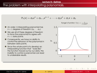
1. Lecture 8—Splines
The problem with interpolating polynomials.
Pn(x) = anxn
+ an−1xn−1
+ · · · + a2x2
+ a1x + a0
An order n interpolating polynomial has
n + 1 degrees of freedom (a0 . . . an).
We use all of these degrees of freedom
to force the polynomial to agree with
n + 1 data points.
Consequently, we have no ability to
control the behavior of the polynomial in
between data points.
Since the whole point is to develop an
interpolating function that ‘‘looks like’’
the function traced out by our data, this
inability to control a polynomial can lead
to undesirable results.
−1 0 1
0
0.5
1
1.5
x1
x
y
Runge’s Function: f(x) = 1
1+25x2
Che 310 | Chapra 18 | Splines 8 — Splines October 24, 2017 1 / 14

2. Lecture 8—Splines
The problem with interpolating polynomials.
Pn(x) = anxn
+ an−1xn−1
+ · · · + a2x2
+ a1x + a0
An order n interpolating polynomial has
n + 1 degrees of freedom (a0 . . . an).
We use all of these degrees of freedom
to force the polynomial to agree with
n + 1 data points.
Consequently, we have no ability to
control the behavior of the polynomial in
between data points.
Since the whole point is to develop an
interpolating function that ‘‘looks like’’
the function traced out by our data, this
inability to control a polynomial can lead
to undesirable results.
−1 0 1
0
0.5
1
1.5
x1
x2
x
y
Runge’s Function: f(x) = 1
1+25x2
Che 310 | Chapra 18 | Splines 8 — Splines October 24, 2017 1 / 14

3. Lecture 8—Splines
The problem with interpolating polynomials.
Pn(x) = anxn
+ an−1xn−1
+ · · · + a2x2
+ a1x + a0
An order n interpolating polynomial has
n + 1 degrees of freedom (a0 . . . an).
We use all of these degrees of freedom
to force the polynomial to agree with
n + 1 data points.
Consequently, we have no ability to
control the behavior of the polynomial in
between data points.
Since the whole point is to develop an
interpolating function that ‘‘looks like’’
the function traced out by our data, this
inability to control a polynomial can lead
to undesirable results.
−1 0 1
0
0.5
1
1.5
x1
x2
x3
x
y
Runge’s Function: f(x) = 1
1+25x2
Che 310 | Chapra 18 | Splines 8 — Splines October 24, 2017 1 / 14

4. Lecture 8—Splines
The problem with interpolating polynomials.
Pn(x) = anxn
+ an−1xn−1
+ · · · + a2x2
+ a1x + a0
An order n interpolating polynomial has
n + 1 degrees of freedom (a0 . . . an).
We use all of these degrees of freedom
to force the polynomial to agree with
n + 1 data points.
Consequently, we have no ability to
control the behavior of the polynomial in
between data points.
Since the whole point is to develop an
interpolating function that ‘‘looks like’’
the function traced out by our data, this
inability to control a polynomial can lead
to undesirable results.
−1 0 1
0
0.5
1
1.5
x1
x2
x3
x4
x
y
Runge’s Function: f(x) = 1
1+25x2
Che 310 | Chapra 18 | Splines 8 — Splines October 24, 2017 1 / 14

5. Lecture 8—Splines
The problem with interpolating polynomials.
Pn(x) = anxn
+ an−1xn−1
+ · · · + a2x2
+ a1x + a0
An order n interpolating polynomial has
n + 1 degrees of freedom (a0 . . . an).
We use all of these degrees of freedom
to force the polynomial to agree with
n + 1 data points.
Consequently, we have no ability to
control the behavior of the polynomial in
between data points.
Since the whole point is to develop an
interpolating function that ‘‘looks like’’
the function traced out by our data, this
inability to control a polynomial can lead
to undesirable results.
−1 0 1
0
0.5
1
1.5
x1
x2
x3
x4x5
x
y
Runge’s Function: f(x) = 1
1+25x2
Che 310 | Chapra 18 | Splines 8 — Splines October 24, 2017 1 / 14

6. Lecture 8—Splines
The problem with interpolating polynomials.
Pn(x) = anxn
+ an−1xn−1
+ · · · + a2x2
+ a1x + a0
An order n interpolating polynomial has
n + 1 degrees of freedom (a0 . . . an).
We use all of these degrees of freedom
to force the polynomial to agree with
n + 1 data points.
Consequently, we have no ability to
control the behavior of the polynomial in
between data points.
Since the whole point is to develop an
interpolating function that ‘‘looks like’’
the function traced out by our data, this
inability to control a polynomial can lead
to undesirable results.
−1 0 1
0
0.5
1
1.5
x1
x2
x3
x4x5
x6
x7 x8
x9
x
y
Runge’s Function: f(x) = 1
1+25x2
Che 310 | Chapra 18 | Splines 8 — Splines October 24, 2017 1 / 14

7. Lecture 8—Splines
The problem with interpolating polynomials.
Pn(x) = anxn
+ an−1xn−1
+ · · · + a2x2
+ a1x + a0
An order n interpolating polynomial has
n + 1 degrees of freedom (a0 . . . an).
We use all of these degrees of freedom
to force the polynomial to agree with
n + 1 data points.
Consequently, we have no ability to
control the behavior of the polynomial in
between data points.
Since the whole point is to develop an
interpolating function that ‘‘looks like’’
the function traced out by our data, this
inability to control a polynomial can lead
to undesirable results.
−1 0 1
0
0.5
1
1.5
x1
x2
x3
x4x5
x6
x7 x8
x9
x
y
Runge’s Function: f(x) = 1
1+25x2
Higher order does not always lead to
higher accuracy.
Che 310 | Chapra 18 | Splines 8 — Splines October 24, 2017 1 / 14

8. Outline
1 Linear algebra application: Piecewise interpolating polynomials
(splines)
Quadratic Splines
Cubic Splines
Che 310 | Chapra 18 | Splines 8 — Splines October 24, 2017 2 / 14

9. Splines — Using our degrees of freedom differently
If we have n + 1 data points, we have at
least n + 1 constraints to use in specifying
an interpolating function.
−0.5 0 0.5
0
0.5
1
x1
x2 x3
x4
Runge’s Function: f(x) = 1
1+25x2
Che 310 | Chapra 18 | Splines 8 — Splines October 24, 2017 3 / 14

10. Splines — Using our degrees of freedom differently
If we have n + 1 data points, we have at
least n + 1 constraints to use in specifying
an interpolating function.
There are n sections defined by the n + 1
points.
−0.5 0 0.5
0
0.5
1
x1
x2 x3
x4
Runge’s Function: f(x) = 1
1+25x2
Che 310 | Chapra 18 | Splines 8 — Splines October 24, 2017 3 / 14

11. Splines — Using our degrees of freedom differently
If we have n + 1 data points, we have at
least n + 1 constraints to use in specifying
an interpolating function.
There are n sections defined by the n + 1
points.
Instead of using a single order n polynomial
to interpolate the data, we could use n
1st-order polynomials:
s
1
i (x) = fi +
fi+1 − fi
xi+1 − xi
(x − x1)
The collection of lines together form the 1st
order interpolating spline
−0.5 0 0.5
0
0.5
1
x1
x2 x3
x4
s
1
1
(x)
s1
2(x)
s 1
3 (x)
Runge’s Function: f(x) = 1
1+25x2
Che 310 | Chapra 18 | Splines 8 — Splines October 24, 2017 3 / 14

12. Splines — Using our degrees of freedom differently
A line has 2 degrees of freedom:
s
1
i (x) = a0 + a1(x − xi )
There are 3 lines, for a total of 6 degrees
freedom.
For each line, s1
i (x), we require that it
agrees with the point on the left side of its
interval:
s
1
i (xi ) = fi
This costs 3 degrees of freedom.
For each line, s1
i (x), we also require that it
agrees with the point on the right side of its
interval:
s
1
i (xi+1) = fi+1
This costs the other 3 degrees of freedom. −0.5 0 0.5
0
0.5
1
x1
x2 x3
x4
s
1
1
(x)
s1
2(x)
s 1
3 (x)
Runge’s Function: f(x) = 1
1+25x2
Che 310 | Chapra 18 | Splines 8 — Splines October 24, 2017 3 / 14

13. Splines — Using our degrees of freedom differently
1st-order splines are not always useful since
they still fail to represent the function
described by the data in between data
points.
−0.5 0 0.5
0
0.5
1
x1
x2 x3
x4
s
1
1
(x)
s1
2(x)
s 1
3 (x)
Runge’s Function: f(x) = 1
1+25x2
Che 310 | Chapra 18 | Splines 8 — Splines October 24, 2017 3 / 14

14. Splines — Using our degrees of freedom differently
1st-order splines are not always useful since
they still fail to represent the function
described by the data in between data
points.
Furthermore, there are ‘‘sharp corners’’
(discontinuous derivatives) where each
segment of the spline meets the next
segment.
−0.5 0 0.5
0
0.5
1
x1
x2 x3
x4
s
1
1
(x)
s1
2(x)
s 1
3 (x)
Runge’s Function: f(x) = 1
1+25x2
Che 310 | Chapra 18 | Splines 8 — Splines October 24, 2017 3 / 14

15. Splines — Using our degrees of freedom differently
1st-order splines are not always useful since
they still fail to represent the function
described by the data in between data
points.
Furthermore, there are ‘‘sharp corners’’
(discontinuous derivatives) where each
segment of the spline meets the next
segment.
To fix this, we can add more degrees of
freedom to our spline. Instead of using lines
to connect the points, we could use
parabolas:
s
2
i (x) = a0 + a1(x − xi ) + a2(x − xi )
2
−0.5 0 0.5
0
0.5
1
x1
x2 x3
x4
s
1
1
(x)
s1
2(x)
s 1
3 (x)
Runge’s Function: f(x) = 1
1+25x2
Che 310 | Chapra 18 | Splines 8 — Splines October 24, 2017 3 / 14

16. Splines — Using our degrees of freedom differently
Each parabola has 3 degrees of freedom.
We have n intervals, for a total of 3n
degrees of freedom.
s
2
i (x) = a0 + a1(x − xi ) + a2(x − xi )
2
We start by drawing any parabola that
connects the first 2 points. This costs 3
degrees of freedom.
−0.5 0 0.5
0
0.5
1
x1
x2 x3
x4
s2
1(x)
Runge’s Function: f(x) = 1
1+25x2
Che 310 | Chapra 18 | Splines 8 — Splines October 24, 2017 3 / 14

17. Splines — Using our degrees of freedom differently
Each parabola has 3 degrees of freedom.
We have n intervals, for a total of 3n
degrees of freedom.
s
2
i (x) = a0 + a1(x − xi ) + a2(x − xi )
2
We start by drawing any parabola that
connects the first 2 points. This costs 3
degrees of freedom.
For the next segment, we require that:
1 s2
2(x2) = f2
2 s2
2(x3) = f3
3 s2
2 (x2) = s2
1 (x2)
The last requirement forces the next
segment to have the same slope as the last
segment where they connect.
−0.5 0 0.5
0
0.5
1
x1
x2 x3
x4
s2
1(x)
s2
2 (x)
Runge’s Function: f(x) = 1
1+25x2
Che 310 | Chapra 18 | Splines 8 — Splines October 24, 2017 3 / 14

18. Splines — Using our degrees of freedom differently
Each parabola has 3 degrees of freedom.
We have n intervals, for a total of 3n
degrees of freedom.
s
2
i (x) = a0 + a1(x − xi ) + a2(x − xi )
2
We start by drawing any parabola that
connects the first 2 points. This costs 3
degrees of freedom.
For the next segment, we require that:
1 s2
2(x2) = f2
2 s2
2(x3) = f3
3 s2
2 (x2) = s2
1 (x2)
The last requirement forces the next
segment to have the same slope as the last
segment where they connect.
We repeat this for each of the remaining
segments.
−0.5 0 0.5
0
0.5
1
x1
x2 x3
x4
s2
1(x)
s2
2 (x)
s
2
3
(x)
Runge’s Function: f(x) = 1
1+25x2
We repeat this for each of the remaining segments.
Che 310 | Chapra 18 | Splines 8 — Splines October 24, 2017 3 / 14

19. How do we determine the spline coefficients?
Using the first constraint, write out the spline equation:
s
2
i (xi ) = ai + bi (xi − xi ) + ci (xi − xi )
2
= fi
ai = fi
Constraints for each spline:
s2
i (x) = ai + bi (x − xi )
h
+ci h2
1 Segment i must agree with the
point on the left:
s
2
i (xi ) = fi
2 Segment i must agree with the
point on the right:
s
2
i (xi+1) = fi+1
3 The derivative of segment i must
agree with that of segment i + 1
at xi+1
s
2
i (xi+1) = s
2
i+1 (xi+1)
Che 310 | Chapra 18 | Splines 8 — Splines October 24, 2017 4 / 14

20. How do we determine the spline coefficients?
Using the first constraint, write out the spline equation:
s
2
i (xi ) = ai + bi (xi − xi ) + ci (xi − xi )
2
= fi
ai = fi
Now write out the second constraint, with hi = xi+1 − xi
s
2
i (xi+1) = fi + bi hi + ci h
2
i+1 = fi+1
fi+1 = fi + bi hi + ci h
2
i+1
Constraints for each spline:
s2
i (x) = ai + bi (x − xi )
h
+ci h2
1 Segment i must agree with the
point on the left:
s
2
i (xi ) = fi
2 Segment i must agree with the
point on the right:
s
2
i (xi+1) = fi+1
3 The derivative of segment i must
agree with that of segment i + 1
at xi+1
s
2
i (xi+1) = s
2
i+1 (xi+1)
Che 310 | Chapra 18 | Splines 8 — Splines October 24, 2017 4 / 14

21. How do we determine the spline coefficients?
Using the first constraint, write out the spline equation:
s
2
i (xi ) = ai + bi (xi − xi ) + ci (xi − xi )
2
= fi
ai = fi
Now write out the second constraint, with hi = xi+1 − xi
s
2
i (xi+1) = fi + bi hi + ci h
2
i+1 = fi+1
fi+1 = fi + bi hi + ci h
2
i+1
Rearrange this last equation:
fi+1 − fi
hi
=
fi+1 − fi
xi+1 − xi
= i = bi + ci hi+1
i = bi + ci hi+1
Constraints for each spline:
s2
i (x) = ai + bi (x − xi )
h
+ci h2
1 Segment i must agree with the
point on the left:
s
2
i (xi ) = fi
2 Segment i must agree with the
point on the right:
s
2
i (xi+1) = fi+1
3 The derivative of segment i must
agree with that of segment i + 1
at xi+1
s
2
i (xi+1) = s
2
i+1 (xi+1)
Che 310 | Chapra 18 | Splines 8 — Splines October 24, 2017 4 / 14

22. How do we determine the spline coefficients?
Using the first constraint, write out the spline equation:
s
2
i (xi ) = ai + bi (xi − xi ) + ci (xi − xi )
2
= fi
ai = fi
Now write out the second constraint, with hi = xi+1 − xi
s
2
i (xi+1) = fi + bi hi + ci h
2
i+1 = fi+1
fi+1 = fi + bi hi + ci h
2
i+1
Rearrange this last equation:
fi+1 − fi
hi
=
fi+1 − fi
xi+1 − xi
= i = bi + ci hi+1
i = bi + ci hi+1
Now write out the third constraint:
bi + 2ci (xi+1 − xi ) = bi+1 + 2ci (xi+1 − xi+1)
ci =
bi+1 − bi
2hi
Constraints for each spline:
s2
i (x) = ai + bi (x − xi )
h
+ci h2
1 Segment i must agree with the
point on the left:
s
2
i (xi ) = fi
2 Segment i must agree with the
point on the right:
s
2
i (xi+1) = fi+1
3 The derivative of segment i must
agree with that of segment i + 1
at xi+1
s
2
i (xi+1) = s
2
i+1 (xi+1)
Che 310 | Chapra 18 | Splines 8 — Splines October 24, 2017 4 / 14

23. How do we determine the spline coefficients?
Insert (3) into (2):
i = bi +
bi+1 − bi
2hi
hi
Important results so far:
s2
i (x) = ai + bi h + ci h2
1
ai = fi
2
i = bi + ci hi
3
ci =
bi+1 − bi
2hi
=
i − bi
hi
Che 310 | Chapra 18 | Splines 8 — Splines October 24, 2017 5 / 14

24. How do we determine the spline coefficients?
Insert (3) into (2):
i = bi +
bi+1 − bi
2hi
hi
The hi cancel:
i = bi +
bi+1 − bi
2
Important results so far:
s2
i (x) = ai + bi h + ci h2
1
ai = fi
2
i = bi + ci hi
3
ci =
bi+1 − bi
2hi
=
i − bi
hi
Che 310 | Chapra 18 | Splines 8 — Splines October 24, 2017 5 / 14

25. How do we determine the spline coefficients?
Insert (3) into (2):
i = bi +
bi+1 − bi
2hi
hi
The hi cancel:
i = bi +
bi+1 − bi
2
So
bi + bi+1
unknown
= 2 i
known
Important results so far:
s2
i (x) = ai + bi h + ci h2
1
ai = fi
2
i = bi + ci hi
3
ci =
bi+1 − bi
2hi
=
i − bi
hi
Che 310 | Chapra 18 | Splines 8 — Splines October 24, 2017 5 / 14

26. How do we determine the spline coefficients?
We can formulate a linear system of equations to find the
bi :
Suppose that we have 4 data points, so we need 3
splines:
b1 +b2 = 2 1
b2 +b3 = 2 2
Important results so far:
s2
i (x) = ai + bi h + ci h2
1
ai = fi
2
bi + bi+1 = 2 i
3
ci =
bi+1 − bi
2hi
=
i − bi
hi
Che 310 | Chapra 18 | Splines 8 — Splines October 24, 2017 6 / 14

27. How do we determine the spline coefficients?
We can formulate a linear system of equations to find the
bi :
Suppose that we have 4 data points, so we need 3
splines:
b1 +b2 = 2 1
b2 +b3 = 2 2
We have 3 unknown bi , but only 2 equations so far. We
can write (2) one more time if we introduce a forth b, b4:
b1 +b2 = 2 1
b2 +b3 = 2 2
b3 +b4 = 2 3
Important results so far:
s2
i (x) = ai + bi h + ci h2
1
ai = fi
2
bi + bi+1 = 2 i
3
ci =
bi+1 − bi
2hi
=
i − bi
hi
Che 310 | Chapra 18 | Splines 8 — Splines October 24, 2017 6 / 14

28. How do we determine the spline coefficients?
Now we have 3 equations and 4
unknowns. The final equation comes
from the fact that the first parabola
we draw can be any parabola that
connects the first two points. We can
choose any value for b1.
b1 = our choice
b1 + b2 = 2 1
b2 + b3 = 2 2
b3 + b4 = 2 3
A common choice is to force the first
segment to be a linear segment:
b1 = 1
Important results so far:
s2
i (x) = ai + bi h + ci h2
1
ai = fi
2
bi + bi+1 = 2 i
3
ci =
bi+1 − bi
2hi
=
i − bi
hi
Che 310 | Chapra 18 | Splines 8 — Splines October 24, 2017 6 / 14

29. Generating a quadratic spline
An example with Runge’s function
Fit Runge’s Function with a 5 data-point spline
First define the data points and the
i and hi:
x = linspace(-1,1,5)’;% Column vector!
y = 1 ./ (1 + 25 .* x.^2);%
clf; hold on;
plot(x,y,’o’);%
5 fplot(@(x)1./(1+25.*x.^2),[-1 1]);%
h = x(2:end) - x(1:end-1);%
nabla = ( y(2:end)- y(1:end-1) ) ./ h;
We have 5 data points. So there
are 4 parabolas for which we must
calculate coefficients.
The constant term is the easiest, just
the first 4 y-values:
a = y(1:end-1); % There are 5 y-values, but only
% the first 4 are used.
% (One per spline segment.)
−1 −0.5 0 0.5 1
0
1
x
y
Che 310 | Chapra 18 | Splines 8 — Splines October 24, 2017 7 / 14

30. Generating a quadratic spline
An example with Runge’s function
Fit Runge’s Function with a 5 data-point spline
The next step is to calculate the linear terms.
These are given by the equations:
b1 + b2 = 2 1 = 2
y2−y1
x2−x1
b2 + b3 = 2 2 = 2
y3−y2
x3−x2
b3 + b4 = 2 3 = 2
y4−y3
x4−x3
b4 + b5 = 2 4 = 2
y5−y4
x5−x4
Where did b5 come from? There are only 4
spline segments in this example.
It turns out that this extra b-value is needed to
calculate the c-value for the last segment:
c4 =
b5 − b4
h4
−1 −0.5 0 0.5 1
0
1
x
y
Che 310 | Chapra 18 | Splines 8 — Splines October 24, 2017 8 / 14

31. Generating a quadratic spline
An example with Runge’s function
Fit Runge’s Function with a 5 data-point spline
The next step is to calculate the linear terms.
These are given by the equations:
b1 = 1
b1 + b2 = 2 1 = 2
y2−y1
x2−x1
b2 + b3 = 2 2 = 2
y3−y2
x3−x2
b3 + b4 = 2 3 = 2
y4−y3
x4−x3
b4 + b5 = 2 4 = 2
y5−y4
x5−x4
Where did b5 come from? There are only 4
spline segments in this example.
It turns out that this extra b-value is needed to
calculate the c-value for the last segment:
c4 =
b5 − b4
h4
So far there are 4 equations but 5 unknown bi
values. This is where we must specify the extra
degree of freedom.
For example, setting b1 = 1 forces the
segment starting at x1 and ending at x2 to be
linear.
−1 −0.5 0 0.5 1
0
1
x
y
Che 310 | Chapra 18 | Splines 8 — Splines October 24, 2017 8 / 14

32. Generating a quadratic spline
An example with Runge’s function
Fit Runge’s Function with a 5 data-point spline
The next step is to calculate the linear terms.
These are given by the equations:





1 0 0 0 0
1 1 0 0 0
0 1 1 0 0
0 0 1 1 0
0 0 0 1 1










b1
b2
b3
b4
b5





=





1
2 1
2 2
2 3
2 4





B = eye(length(x));%
for ii = 2:length(x)
B(ii,ii-1) = 1;
end;%
5 rhs = [ nabla(1) ; 2*nabla ];%
b = B rhs; % Remember, b has 5 elements although there are
% only 4 spline segments.
−1 −0.5 0 0.5 1
0
1
x
y
Che 310 | Chapra 18 | Splines 8 — Splines October 24, 2017 8 / 14

33. Generating a quadratic spline
An example with Runge’s function
Fit Runge’s Function with a 5 data-point spline
Finally, the ci parameters can be
calculated using:
ci = i − bi
hi
% Remember, there are 5 b-values but only 4 spline
% segments.
c = (nabla - b(1:end-1)) ./ h;
% Collect all of the coefficients
5 % (the MATLAB piecewise-polynomial
% format calls them ’coefs’ )
coefs = [ c b(1:end-1) a ]; %
−1 0 1
0
1
x1
x2
x3
x4
x5
xy
Che 310 | Chapra 18 | Splines 8 — Splines October 24, 2017 9 / 14

34. Generating a quadratic spline
An example with Runge’s function
Fit Runge’s Function with a 5 data-point spline
Each row of S contains the polynomial
coefficients in Matlab format. For a point
x, the proper row is determined by the
original x-data:
If x < x2, then plot using the first row
of S:
x = linspace(-1.25,-0.5);%
s1 = polyval(S(1,1:3),x-S(1,4));%
plot(x,s1,’r’);
−1 0 1
0
1
x1
x2
x3
x4
x5
xy
Che 310 | Chapra 18 | Splines 8 — Splines October 24, 2017 9 / 14

35. Generating a quadratic spline
An example with Runge’s function
Fit Runge’s Function with a 5 data-point spline
Each row of S contains the polynomial
coefficients in Matlab format. For a point
x, the proper row is determined by the
original x-data:
If x ≥ xi and x < xi+1, use row i:
% From x_2 to x_3
x = linspace(-0.5,0.0);%
s1 = polyval(S(2,1:3),x-S(2,4);%
plot(x,s1,’g’);
5 % From x_3 to x_4
x = linspace(0.,0.5);%
s1 = polyval(S(3,1:3),x-S(3,4);%
plot(x,s1,’g’);
−1 0 1
0
1
x1
x2
x3
x4
x5
xy
Che 310 | Chapra 18 | Splines 8 — Splines October 24, 2017 9 / 14

36. Generating a quadratic spline
An example with Runge’s function
Fit Runge’s Function with a 5 data-point spline
Each row of S contains the polynomial
coefficients in Matlab format. For a point
x, the proper row is determined by the
original x-data:
If x > x4, use row 4:
x = linspace(0.5,1.1);%
s1 = polyval(S(4,1:3),x-S(4,4));%
plot(x,s1,’r’);
−1 0 1
0
1
x1
x2
x3
x4
x5
xy
Che 310 | Chapra 18 | Splines 8 — Splines October 24, 2017 9 / 14

37. Generating a quadratic spline
An example with Runge’s function
Fit Runge’s Function with a 5 data-point spline
Matlab can simplify evaluation of splines
using it’s ‘‘Piecewise polynomial’’
processing functions:
% Transfer the spline data into Matlab’s
% ’pp’ data structure
% mkpp - Make Piecewise Polynomial
my_spline = mkpp(x,coefs);
5 % Use the ppval command to evaluate the spline anywhere
fplot(@(x)ppval(my_spline,x),xlim);
−1 0 1
0
1
x1
x2
x3
x4
x5
xy
Che 310 | Chapra 18 | Splines 8 — Splines October 24, 2017 9 / 14

38. Outline
1 Linear algebra application: Piecewise interpolating polynomials
(splines)
Quadratic Splines
Cubic Splines
Che 310 | Chapra 18 | Splines 8 — Splines October 24, 2017 10 / 14

39. Cubic splines — the interpolation method of choice
Quadratic splines often fail to reproduce the original function in between
data points because the curvature of the parabolas (si (x)) are
mismatched.
Cubic splines fix this problem by adding an additional degree of freedom
Cubic splines: Use 4 degrees of freedom to interpolate between only 2 points
si(x) = a + b(x − xi) + c(x − xi)2
+ d(x − xi)3
Constraints:
1 si(xi) = f(xi) (Interpolates the left point)
2 si(xi+1) = f(xi+1) (Interpolates the right point)
3 si
(xi+1) = si+1
(xi+1) (Continuous derivatives)
4 si
(xi+1) = si+1
(xi+1) (Continuous curvature)
Constraints 3 and 4 ensure that each spline segment smoothly connects
with its neighbors.
Che 310 | Chapra 18 | Splines 8 — Splines October 24, 2017 11 / 14

40. Cubic Splines
Degrees of freedom
Suppose there are n data points.
0.5 1 1.5 2 2.5 3 3.5 4 4.5
−0.5
0
0.5
1
1.5
s1
4 constraints
s2
4 constraints
s3
Only 2 constraints!
x1
x2
x3
x4
x
y
4 data points, 3 spline segments = 12 DOFs
Che 310 | Chapra 18 | Splines 8 — Splines October 24, 2017 12 / 14

41. Cubic Splines
Degrees of freedom
Suppose there are n data points.
Then there are n − 1 cubic polynomials connecting them
0.5 1 1.5 2 2.5 3 3.5 4 4.5
−0.5
0
0.5
1
1.5
s1
4 constraints
s2
4 constraints
s3
Only 2 constraints!
x1
x2
x3
x4
x
y
4 data points, 3 spline segments = 12 DOFs
Che 310 | Chapra 18 | Splines 8 — Splines October 24, 2017 12 / 14

42. Cubic Splines
Degrees of freedom
Suppose there are n data points.
Then there are n − 1 cubic polynomials connecting them
Each cubic polynomial has 4 degrees of freedom
0.5 1 1.5 2 2.5 3 3.5 4 4.5
−0.5
0
0.5
1
1.5
s1
4 constraints
s2
4 constraints
s3
Only 2 constraints!
x1
x2
x3
x4
x
y
4 data points, 3 spline segments = 12 DOFs
Che 310 | Chapra 18 | Splines 8 — Splines October 24, 2017 12 / 14

43. Cubic Splines
Degrees of freedom
Suppose there are n data points.
Then there are n − 1 cubic polynomials connecting them
Each cubic polynomial has 4 degrees of freedom
The first n − 2 segments are subject to 4 constraints.
0.5 1 1.5 2 2.5 3 3.5 4 4.5
−0.5
0
0.5
1
1.5
s1
4 constraints
s2
4 constraints
s3
Only 2 constraints!
x1
x2
x3
x4
x
y
4 data points, 3 spline segments = 12 DOFs
Che 310 | Chapra 18 | Splines 8 — Splines October 24, 2017 12 / 14

44. Cubic Splines
Degrees of freedom
Suppose there are n data points.
Then there are n − 1 cubic polynomials connecting them
Each cubic polynomial has 4 degrees of freedom
The first n − 2 segments are subject to 4 constraints.
The last segment must satisfy only (1) and (2) — there is no next segment
with which to match s and s
0.5 1 1.5 2 2.5 3 3.5 4 4.5
−0.5
0
0.5
1
1.5
s1
4 constraints
s2
4 constraints
s3
Only 2 constraints!
x1
x2
x3
x4
x
y
4 data points, 3 spline segments = 12 DOFs
Che 310 | Chapra 18 | Splines 8 — Splines October 24, 2017 12 / 14

45. Cubic Splines
Degrees of freedom
Suppose there are n data points.
Then there are n − 1 cubic polynomials connecting them
Each cubic polynomial has 4 degrees of freedom
The first n − 2 segments are subject to 4 constraints.
The last segment must satisfy only (1) and (2) — there is no next segment
with which to match s and s
Total DOFS = 4(n − 1)
0.5 1 1.5 2 2.5 3 3.5 4 4.5
−0.5
0
0.5
1
1.5
s1
4 constraints
s2
4 constraints
s3
Only 2 constraints!
x1
x2
x3
x4
x
y
4 data points, 3 spline segments = 12 DOFs
Che 310 | Chapra 18 | Splines 8 — Splines October 24, 2017 12 / 14

46. Cubic Splines
Degrees of freedom
Suppose there are n data points.
Then there are n − 1 cubic polynomials connecting them
Each cubic polynomial has 4 degrees of freedom
The first n − 2 segments are subject to 4 constraints.
The last segment must satisfy only (1) and (2) — there is no next segment
with which to match s and s
Total DOFS = 4(n − 1)
Total constraints = 4(n − 2) + 2 ⇒
A cubic spline requires 2 additional constraints
0.5 1 1.5 2 2.5 3 3.5 4 4.5
−0.5
0
0.5
1
1.5
s1
4 constraints
s2
4 constraints
s3
Only 2 constraints!
x1
x2
x3
x4
x
y
4 data points, 3 spline segments = 12 DOFs
Che 310 | Chapra 18 | Splines 8 — Splines October 24, 2017 12 / 14

47. Cubic Splines
Three common types — Differentiated by how the 2 constraints are chosen
Natural Splines
Second derivative is 0
at first and last points
c1 = cn = 0
−1 −0.5 0 0.5 1
0
0.5
1
x1
x2
x3
x4
x5
Data
Spline
Clamped Splines
Specify the first
derivative is at the
first and last points
−1 −0.5 0 0.5 1
0
0.5
1
x1
x2
x3
x4
x5
s
1(x1)=1
sn
(xn+1
)=−1
Data
Spline
Not-a-knot Splines
Force continuity of third
derivative for the first and last
segments:
s1 (x2) = s2 (x2)
and
sn (xn) = sn−1(xn)
−1 −0.5 0 0.5 1
0
0.5
1
x1
x2
x3
x4
x5
Data
Spline
Che 310 | Chapra 18 | Splines 8 — Splines October 24, 2017 13 / 14

48. The cubic spline equations
For a spline based on n data points there are n − 1 spline segments:
1 ai = f(xi)
Che 310 | Chapra 18 | Splines 8 — Splines October 24, 2017 14 / 14

49. The cubic spline equations
For a spline based on n data points there are n − 1 spline segments:
1 ai = f(xi)
2 n − 2 linear equations for the ci’s:
hi−1ci−1 + 2(hi−1 + hi)ci + hici+1 = 3( i − i−1)
Che 310 | Chapra 18 | Splines 8 — Splines October 24, 2017 14 / 14

50. The cubic spline equations
For a spline based on n data points there are n − 1 spline segments:
1 ai = f(xi)
2 n − 2 linear equations for the ci’s:
hi−1ci−1 + 2(hi−1 + hi)ci + hici+1 = 3( i − i−1)
3 Two linear equations for c1 and cn using spline conditions:
Che 310 | Chapra 18 | Splines 8 — Splines October 24, 2017 14 / 14

51. The cubic spline equations
For a spline based on n data points there are n − 1 spline segments:
1 ai = f(xi)
2 n − 2 linear equations for the ci’s:
hi−1ci−1 + 2(hi−1 + hi)ci + hici+1 = 3( i − i−1)
3 Two linear equations for c1 and cn using spline conditions:
Natural c1 = cn = 0
Che 310 | Chapra 18 | Splines 8 — Splines October 24, 2017 14 / 14

52. The cubic spline equations
For a spline based on n data points there are n − 1 spline segments:
1 ai = f(xi)
2 n − 2 linear equations for the ci’s:
hi−1ci−1 + 2(hi−1 + hi)ci + hici+1 = 3( i − i−1)
3 Two linear equations for c1 and cn using spline conditions:
Natural c1 = cn = 0
Clamped The user specifies the spline derivatives f1 and fn at x1 and
xn
2h1c1 + h1c2 = 3( 1 − f1)
hn−1cn−1 + 2hn−1cn = 3(fn − n)
Che 310 | Chapra 18 | Splines 8 — Splines October 24, 2017 14 / 14

53. The cubic spline equations
For a spline based on n data points there are n − 1 spline segments:
1 ai = f(xi)
2 n − 2 linear equations for the ci’s:
hi−1ci−1 + 2(hi−1 + hi)ci + hici+1 = 3( i − i−1)
3 Two linear equations for c1 and cn using spline conditions:
Natural c1 = cn = 0
Clamped The user specifies the spline derivatives f1 and fn at x1 and
xn
2h1c1 + h1c2 = 3( 1 − f1)
hn−1cn−1 + 2hn−1cn = 3(fn − n)
Not-a-knot
h2c1 − (h1 + h2)c2 + h1c3 = 0
hn−1cn−2 − (hn−2 + hn−1)cn−1 + hn−2cn = 0
Che 310 | Chapra 18 | Splines 8 — Splines October 24, 2017 14 / 14

54. The cubic spline equations
For a spline based on n data points there are n − 1 spline segments:
1 ai = f(xi)
2 n − 2 linear equations for the ci’s:
hi−1ci−1 + 2(hi−1 + hi)ci + hici+1 = 3( i − i−1)
3 Two linear equations for c1 and cn using spline conditions:
Natural c1 = cn = 0
Clamped The user specifies the spline derivatives f1 and fn at x1 and
xn
2h1c1 + h1c2 = 3( 1 − f1)
hn−1cn−1 + 2hn−1cn = 3(fn − n)
Not-a-knot
h2c1 − (h1 + h2)c2 + h1c3 = 0
hn−1cn−2 − (hn−2 + hn−1)cn−1 + hn−2cn = 0
With known ci’s,
bi = i −
hi
3
(ci+1 + 2ci)
di =
1
3hi
(ci+1 − ci)
Che 310 | Chapra 18 | Splines 8 — Splines October 24, 2017 14 / 14