A combination of ball events and positional data is needed to understand the players’ and team’s performance. Thus, several indicators such as player-player and player-ball dyadic coordination, intra-and inter-team synchronization, pattern-forming dynamics, time required to regain ball possession, ball possession percentage, number of passes and their length have been used to characterize individual and collective performance using AI algorithms

1. Studying the effect of Space in the outcome at the end
of possession using Backpropagation algorithm
Now a days data has been widely used in the Performance analysis to give the insight to
coaches about the important information in sport. Performance Analysis has helped in
identifying the parameters of execution, like tactical change in the playing behaviour of team
or how the defensive events are different for an attacking team or a defensive team. These
events have helped in categorizing the style of team and their performance. Though the
previous research gave information about the performance to some extent but still there are
many things to explore . For example, Location of the ball with respect to the scoring targets
constrains the emergence of spatiotemporal coordinated team behaviours (Travassos, B., et
al. , 2019). There has been lot of studies going on to measure the trajectories of the players,
acceleration, cutting movements, space around them or velocities as variable. It helped in
defining the pattern at different levels of analysis (i.e., team , player or game). Therefore,
capturing contextual information is the key challenge in performance analysis which can be
used to analyse the different game scenarios applied by the players and the team.
A combination of ball events and positional data is needed to understand the players’ and
team’s performance. Thus, several indicators such as player-player and player-ball dyadic
coordination, intra-and inter-team synchronization, pattern-forming dynamics, time required
to regain ball possession, ball possession percentage, number of passes and their length have
been used to characterize individual and collective performance (Travassos, B., et al. , 2019).
Network science is the most researched filled in applied physics and mathematics. Though
there are various applications of neural networks we are only interested using it in football.
The nature of the neural network allows catering to different sections of the team
organization and Performance which is generally not identified by regular analysis. The reason
behind relies on the complex nature of the game, which, paraphrasing the foundational
paradigm of complexity sciences “cannot be analysed by looking at its components (i.e.,
players) individually but, on the contrary, considering the system as a whole” or, in the
classical words of after-match interviews “it's not just me, it's the team.”
Neural network is used to recognise pattern which is based on the algorithm applied on it to
train and generate the output. Majorly, the two types of Neural Network used are Supervised
learning and Unsupervised learning. In Supervised learning, system is trained with the
information available to predict the desired output. When the predicted output doesn’t
match the actual output, the difference between them is used to modify the parameter to
reduce the difference and generate better output with lesser error. Multilayer perceptron is
one of the most popular Supervise neural network.
On the other hand the unsupervised learning, the output is still produced on the basis of the
prior assumptions however, the output is not known
Backpropagation, is one of the most popular method of artificial neural networks. it calculates
the gradient of a loss function with respects to all the weights in the network. The gradient is
fed to the optimization method which in turn uses it to update the weights, in an attempt to
minimize the loss function.

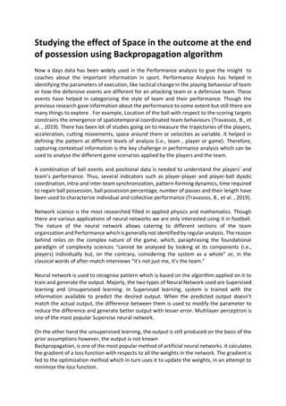
2. Fig 1. Schematic representation of Neural Networks
The following steps is the recursive definition of algorithm:
Step:-
1. Initial weights are chosen randomly
2. Inputs are applied to the network for each training pattern
3. Output is calculated for every neuron from the input layer, through the hidden layer(s), to
the output layer.
4. Error is calculated at the output
Advantages
1. Simple, fast, easy to program.
2. No tuning of parameter is required.
3. Prior knowledge is not required about the weak learner hence can be flexible.
Disadvantages
1. The input data determines the performance of the algorithm
2. Backpropagation can be sensitive to noisy data and outliers.
Data sources
The data being used here is from the Cardiff city Vs Hull match. There are different files with
different variable.
System Specification
Prozone has provided X and Y coordinates of all the players for each tenth of a second. The
center of the circle is taken as (0,0). The positive X goes from left to right and the positive Y
goes from top to bottom. There are total 54000 rows for whole 90 minutes.
The other file is an event file has seven columns which store a record for each instantaneous
event performed during the match.
The 7 column of event files are
1. Half (1 or 2)
2. Mins (on video)
3. Seconds (on video)
4. Team (1 = Hull, 2 = Cardiff)
5. Player (1 to 26, 1 to 12 are the Hull players, 13 to 26 are the Cardiff players, 0 = N/A)
6. Event (1 = Pass, 2 = Receive, 3 = Touch, 4 = Shot, 5 = Corner, 6 = Throw In, 0 = N/A)
7. Outcome (1 = Retained, 2 = Lost, 0 = N/A)
Inputs
Output
x1
w1
x2
w2
x3
w3
f( wixi)

3. PROCESSING THE DATA
Artificial neural networks
Artificial neural networks trained to recognise complex patterns, classifying these patterns
using supervised or unsupervised learning algorithms. This section describes the use of
artificial neural networks to recognise tactical patterns associated with successful
possessions. A simple example is used where 392 possessions from a single English FA
Premier League match are analysed. There were 26 players who participated in the match.
However, the data were pre-processed so that only the 22 players on the pitch were
represented for any instant in the game. This meant that where a player was substituted, a
single pair of columns (X and Y) represented the player and the substitute once he entered
the field. The player co-ordinates were recorded using a commercial automatic player
tracking system (Prozone3: Prozone Sports Ltd, Leeds, UK). The artificial neural networks use
the difference of distance between the player with the ball and all the player of opposite team
at the start of possession and at the end. Knowing the player in possession of the ball at the
start of each possession also allowed the location of the ball at the start of each possession
and the loosing of possession helped in determining the player who lost the ball. Possession
outcomes are classified as successful if there is a scoring opportunity or the attacking team
enters the attacking third (n = 122), otherwise they are classed as unsuccessful (n = 294). The
times at which possessions commenced as well as the outcomes of possessions were
determined using a manual video analysis process
Possession
Using the event file, a new possession file was created. The main aim was to find the player
losing the ball at the end of possession because if we have the player at the start and end of
possession we can calculate the distance at the start and end with the players of opposition
team. There were some cases when the ball went out was not in play. We have assumed here
that the possession continues if the ball is still with the team who had the ball previously
before the ball went out.
Backpropagation algorithm
Here we are going to compare the two different feedforward networks. One with 1 hidden
player and one with two hidden layer. The middle layer used the ‘ReLu’ transfer function
whereas the output layer used the ‘Softmax’ as the output function. The data was split into
testing and training data in the ration of 70 % -30 %. The weights were initialised randomly.
In the first case with only 1 middle layer A range of middle layer sizes were studied for each
neural network type with the neural networks being trained using the backpropagation
algorithm. In the second case with two middle layer, one layer was kept at constant 50 while
the other layer’s size was changed from 10 to 50 (10,20,30,40,50) to see the effect
The system studied the two networks to iterate the train-test of neural network 500 times for
each layer. The system runs twice for both the cases. The output obtained was in categorical
terms hence three different output layers needed for them. There is no case of overlap as the
output was categorized in 1,0,0 format.

4. Space:
Space around a player can reported in different formats. For example, like calculating the area
using the Voronoi diagram or by calculating the distance of player from the goal when the
possession starts. Distances can also be computed between pairs of players on the same
team, between opposing players, or between players and the ball. Here we have used the
distance between the player with the ball and all the players of opposite team. This is distance
is calculated at the start and at the end of possession. The difference of this distance is used
to analyse its effect on the outcome.
Imbalance Data :
Data being used here is an imbalance data, which means the percentage of one type of
outcome is skewed in favour of one output. Therefore the accuracy metrics won’t be the
right way of evaluation of the model.
Outcome Training Cases Test Cases All Cases
Unsuccessful 186 97 283
Last third no scoring
opportunity
58 28 86
Scoring opportunity 18 5 23
Total 262 130 392
Table 1. Showing the distribution of outcome in training and test case.
Results
Now, if we talk about the difference of the distances. For every instances there will be 11
difference of the distance. When the number of distance negative is less than or equal to 3 it
is termed as Low(green box), if it is between 4-7 then medium(yellow box) and >7 it is high(red
box). When the number of negative is higher it means that distance has decreased with more
than 7 players at the of possession and it means the player is moving to attack or it is being
pressed by the opposite team. Now, if see the blue bar in case of high numbers, it’s the
smallest hence it means that the opposite team have style of pressing the game and not
sitting back and defending.
Fig 2. Showing the difference of the distance at the start and end of possession

5. Fig 3. Showing distribution of outcome on the basis of difference of distance
10 20 30 40 50
Test Accuracy 66.92 67.69 63.85 75.38 69.23
Train Accuracy 99.24 99.62 99.24 97.71 100.00
Average
Precision : 0.46 0.45 0.40 0.61 0.53
Average recall : 0.56 0.46 0.40 0.58 0.53
Average f1 : 0.49 0.45 0.40 0.58 0.53
Table 2. showing the values for one middle layer(1M)
10 20 30 40 50
Test Accuracy 63.08 75.38 58.46 65.38 64.62
Train Accuracy 100.00 100.00 100.00 100.00 100.00
Average
Precision : 0.41 0.59 0.35 0.42 0.38
Average recall : 0.40 0.48 0.37 0.41 0.37
Average f1 : 0.40 0.51 0.35 0.42 Nan
Table 3. showing the values for two middle layer(2M)
Discussion
On each occasion, 262 new possessions were used to train the network and the other 130
possessions were used to test the predictive accuracy of the network. The system recorded
accuracy, Recall(sensitivity) and Precision(specificity )statistics for each train-test cycle
allowing mean values for each combination of network type and middle layer size to be
determined. Accuracy is the percentage of all possessions for which the neural network
predicted the correct outcome. Recall is the percentage of successful possessions where the
neural network correctly predicted a successful outcome. Precision is the percentage of
unsuccessful possessions where the neural network correctly predicted an unsuccessful

6. outcome. (Snow, P., et al. , 1994). During each train-test cycle, the input vector was set up
using the difference of the distances at the start of that particular possession and the end of
it. Possession end here is considered when the upcoming events is not retained by the same
team. The target outcome was copied from the original data for the 262 training cases.
As mentioned, the network was trained with 262 randomly selected possessions during each
train-test cycle. Within each cycle, the remaining 130 cases were used to test the accuracy of
the trained network. This was done by using the keras library. The layers were setup for input
and output. Since this is a classification problem, the output layers has 3 nodes one for each
category of output. As each possession was tested, accuracy, Recall and precision statistics
were determined.
The accuracy levels of both the cases are similar. In the first case with one middle layer, the
test accuracy is highest when there are 50 nodes in the layer but the test accuracy is not that
good. When the nodes are 40, the test accuracy is highest and the difference between the
test accuracy and training accuracy is lowest. Higher training accuracy and lower test accuracy
means that model is overfitting hence we have to find a sweet spot where it is not overfitting
and also performing well on the unseen data. For 1-Middle layer the best combination is one
layer with 40 nodes whereas for the second layer one layer is with 50 and the other is 20
nodes for the best results
Fig 4. On left, showing the training and test accuracy with 1 middle layer and on the right with 2 middle
layer
If we talk about precision,
Precision is highest for the Two middle layer system when the second layer has 20 nodes is
with highest precision. Test accuracy was also the highest for the same number of nodes.
For 1M layer, when the second layer has 40 nodes is with highest precision. Test
accuracy was also the highest for the same number of nodes.
Fig 5. Comparing precision for 1M layer and 2M layer
0
100
200
10 20 30 40 50
One Middle layer
Test Accuracy Train Accuracy
0
100
200
10 20 30 40 50
Two Middle layer
Test Accuracy Train Accuracy
0
0.2
0.4
0.6
0.8
1 2 3 4 5
Average precision
Average Precision(1M) : Average Precision(2M) :

7. In case of Recall, the 40 nodes for 1M layer has the highest value whereas for the 2M layer,
when the second middle layer has 20 nodes has the highest value.
Fig 6. Comparing Average Recall for 1M layer and 2M layer
It is important to consider the contribution of false positive and false negative predictions in
selecting the best neural network structure to use rather than just looking at the overall
accuracy level.
A disappointing aspect of both neural network performances was the tendency to predict
outcome of possessions largely on the basis of X co-ordinate of the attacking team. All of the
possessions predicted to be successful were located in the other team’s half of the pitch
despite the clear overlap of locations of possessions of different outcomes. An explanation
for the apparent mechanical classification of possessions is the quantitative nature of the pre-
processed data used. Neural networks were designed to be used with more complex pattern-
like data (Lamb and Bartlett, 2013; Perl et al., 2013). It should also be considered that a one-
frame snapshot of a possession is very limited information and the outcomes of possessions
also depend on behaviours beyond this instant in time. A further explanation for the lack of
accuracy in recognising successful possessions that started in the team’s own half is due to
the nature of sports performance. The neural network may recognise situations where teams
have a greater opportunity of success than other situations, but in reality there are occasions
where teams achieve successful outcomes that were not likely and other occasions where
they fail to achieve successful outcomes despite being in a favourable situation.
Conclusions
There is a vast amount of spatio-temporal data that can be gathered during sports
performance using player tracking technology. These data can be analysed using algorithmic
techniques or artificial intelligence. Algorithmic approaches are challenging in that they
require analysts to specify aspects of play in a mathematical form that covers all cases of the
given tactic being identified. This is not really possible and so analysts need to have strategies
to identify and deal with false positive and false negative predictions by algorithms. Artificial
neural networks can undergo supervised learning to distinguish possessions of differing
outcomes. As before, there will be false positive and false negative predictions made. A
further issue is that while weights within trained artificial neural networks can be inspected,
the mechanisms by which they predict the success of possessions are not as transparent as
the way in which analyst written algorithms distinguish between different tactics.
Unsupervised learning is an alternative approach that can lead to the identification of
possession types not considered by the analyst but which may be associated with success
0
0.1
0.2
0.3
0.4
0.5
0.6
0.7
1 2 3 4 5
Average Recall
Average recall(2M) Average recall(1M) :

8. References
1. Travassos, B., Araújo, D., Duarte, R. and McGarry, T. (2019). Spatiotemporal
coordination behaviors in futsal (indoor football) are guided by informational game
constraints.
2. Snow, P., Smith, D. and Catalona, W. (1994). Artificial Neural Networks in the Diagnosis
and Prognosis of Prostate Cancer: A Pilot Study. Journal of Urology, 152(5 Part 2),
pp.1923-1926.
3. Lamb, P. and Bartlett, R. (2013), Neural networks for analysing sports techniques, In
T. McGarry, P. O’Donoghue and J. Sampaio (eds.), Routledge Handbook of Sports
Performance Analysis (pp. 225-236), London: Routledge.