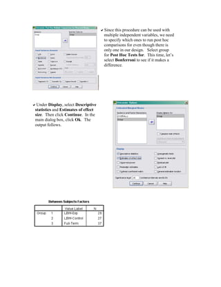
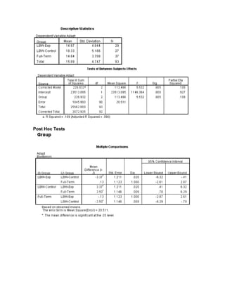
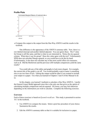
8. Comparing Means Using One Way
ANOVA
Objectives
Calculate a one-way analysis of variance
Run various multiple comparisons
Calculate measures of effect size
A One Way ANOVA is an analysis of variance in which there is only one
independent variable. It can be used to compare mean differences in 2 or more groups.
In SPSS, you can calculate one-way ANOVAS in two different ways. One way is
through Analyze/Compare Means/One-Way ANOVA and the other is through
Analyze/General Linear Model/Univariate. We’ll try both in this chapter so we can
compare them.
One-Way ANOVA
Let’s begin with an example in the textbook illustrated in Table 16.6. Maternal
role adaptation was compared in a group of mothers of low birth-weight (LBW) infants
who had been in an experimental intervention, mothers of LBW infants who were in a
control group, and mothers of full-term infants. The hypothesis was that mothers of
LBW infants in the experimental intervention would adapt to their maternal role as well
as mothers of healthy full-term infants, and each of these groups would adapt better than
mothers of LBW infants in the control group.
Open maternal role adaptation.sav.
Select Analyze/Compare Means/One-Way ANOVA.
Select maternal role adaptation for the
Dependent List since it is the dependent
variable. Select group as the Factor or
independent variable. Then click Post Hoc to
see various options for calculating multiple
comparisons. If the ANOVA is significant,
we can use the post hoc tests to determine
which specific groups differ significantly
from one another.
Note that .05 is the default under Significance level. After consulting with SPSS
technical support, it is clear that this is the experiment-wise or family-wise significance
level. So any comparison flagged by SPSS as significant is based on a Bonferroni
Type Correction. You do not need to adjust the significance level yourself.
As you can see, there are
many options. Let’s select
LSD under Equal Variances
Assumed since it is Fisher’s
Least Significant Difference
Test which is calculated in the
text, except that SPSS will test
the differences even if the
overall F is not significant.
Click Options. In the next dialog box, select
Descriptives under Statistics, and select Means plot
so SPSS will create a graph of the group means for us.
The default under Missing Values is Exclude cases
analysis by analysis. Let’s leave this as is. Click
Continue and then Ok. The output follows.
Means Plots
GROUP
Full-termLBW ControlLBW Experimental
19
18
17
16
15
14
Compare this output to the results presented in the text.
We can see the descriptive statistics and the F value are the same. It is harder to
compare the post hoc comparisons because SPSS does not display the t values. They
simply report the mean difference and the significance level. The important thing to note
is that the conclusions we can draw based on each of these approaches are the same.
The plot that SPSS created is an effective way to illustrate the mean differences.
You may want to edit the graph using what you learned in Chapter 3 to make it more
elegant. Some people would prefer a bar chart since these are independent groups and a
line suggests they are related. You could create a bar chart of these group means
yourself.
Let’s re-run the same analysis using the General Linear Model (GLM) and see
how they are similar and different.
General Linear Model to Calculate One-Way ANOVAs
The Univariate General Linear Model is really intended to test models in which
there is one dependent variable and multiple independent variables. We can use it to run
a simple one-way ANOVA like the one above. One advantage of doing so is that we can
estimate effect size from this menu, but we could not from the One-Way ANOVA menus.
Let’s try it.
Select Analyze/General Linear Model/Univariate.
As you can see by this dialog box, there
are many more options than the One-
Way ANOVA. This is because the
GLM is a powerful technique that can
examine complex designs. We’ll just
focus on what is relevant to us. As
before, select maternal role adaptation
as the Dependent Variable and group
as the Fixed Factor or independent
variable. Then, click Plots.
Select group for the Horizontal Axis (X axis),
and click add. Since there is only one dependent
variable, SPSS knows that maternal role
adaptation is on the Y axis without us needing the
specify this. Click Continue.
Since this procedure can be used with
multiple independent variables, we need
to specify which ones to run post hoc
comparisons for even though there is
only one in our design. Select group
for Post Hoc Tests for. This time, let’s
select Bonferroni to see if it makes a
difference.
Under Display, select Descriptive
statistics and Estimates of effect
size. Then click Continue. In the
main dialog box, click Ok. The
output follows.
Post Hoc Tests
Profile Plots
Estimated Marginal Means of maternal role adaptation (low sores better)
GROUP
Full-termLBW ControlLBW Experimental
EstimatedMarginalMeans
19
18
17
16
15
14
Compare this output to the output from the One-Way ANOVA and the results in the
textbook.
One difference is the appearance of the ANOVA summary table. Now, there is a
row labeled intercept and another labeled adjusted. You can ignore these. The F value
for Group is still the same, and that is what we are interested in. Notice the eta squared
column. What does it say for group? Does this value agree with the text? Unfortunately
SPSS does not calculate Omega squared, so you would have to do this by hand.
(Unfortunately, it also does not calculate any of the more useful effect size measures,
such as d. Did the Bonferroni and the previous LSD multiple comparisons yield the same
results?
You could edit any of the tables and graphs to look more elegant. For example,
the current title of the graph is cut off. You would probably want to name it something
else or use two lines of text. Editing the output would be ideal if you wanted to include
your output in a paper. Use what you learned in Chapters 3 and 4 of this Manual to do
so.
In this chapter, you learned 3 methods to calculate a One-Way ANOVA. I prefer
the General Linear Model approach since this is the only one that gives us the option of
calculating multiple comparisons and eta squared. Of course, you may feel otherwise
depending on the information you wish to calculate. Complete the following exercises.
Exercises
Each of these exercises is based on Eysenck recall.sav. This study is presented in section
16.1 in the textbook.
1. Use ANOVA to compare the means. Select a post hoc procedure of your choice.
Summarize the results.
2. Edit the ANOVA summary table so that it is suitable for inclusion in a paper.
3. Use SPSS to calculate eta squared. Note, how did you do this?
4. Create a bar chart to illustrate the differences between groups.

One way anova

  • 1.
    8. Comparing MeansUsing One Way ANOVA Objectives Calculate a one-way analysis of variance Run various multiple comparisons Calculate measures of effect size A One Way ANOVA is an analysis of variance in which there is only one independent variable. It can be used to compare mean differences in 2 or more groups. In SPSS, you can calculate one-way ANOVAS in two different ways. One way is through Analyze/Compare Means/One-Way ANOVA and the other is through Analyze/General Linear Model/Univariate. We’ll try both in this chapter so we can compare them. One-Way ANOVA Let’s begin with an example in the textbook illustrated in Table 16.6. Maternal role adaptation was compared in a group of mothers of low birth-weight (LBW) infants who had been in an experimental intervention, mothers of LBW infants who were in a control group, and mothers of full-term infants. The hypothesis was that mothers of LBW infants in the experimental intervention would adapt to their maternal role as well as mothers of healthy full-term infants, and each of these groups would adapt better than mothers of LBW infants in the control group. Open maternal role adaptation.sav. Select Analyze/Compare Means/One-Way ANOVA. Select maternal role adaptation for the Dependent List since it is the dependent variable. Select group as the Factor or independent variable. Then click Post Hoc to see various options for calculating multiple comparisons. If the ANOVA is significant, we can use the post hoc tests to determine which specific groups differ significantly from one another.
  • 2.
    Note that .05is the default under Significance level. After consulting with SPSS technical support, it is clear that this is the experiment-wise or family-wise significance level. So any comparison flagged by SPSS as significant is based on a Bonferroni Type Correction. You do not need to adjust the significance level yourself. As you can see, there are many options. Let’s select LSD under Equal Variances Assumed since it is Fisher’s Least Significant Difference Test which is calculated in the text, except that SPSS will test the differences even if the overall F is not significant. Click Options. In the next dialog box, select Descriptives under Statistics, and select Means plot so SPSS will create a graph of the group means for us. The default under Missing Values is Exclude cases analysis by analysis. Let’s leave this as is. Click Continue and then Ok. The output follows.
  • 3.
    Means Plots GROUP Full-termLBW ControlLBWExperimental 19 18 17 16 15 14 Compare this output to the results presented in the text. We can see the descriptive statistics and the F value are the same. It is harder to compare the post hoc comparisons because SPSS does not display the t values. They simply report the mean difference and the significance level. The important thing to note is that the conclusions we can draw based on each of these approaches are the same.
  • 4.
    The plot thatSPSS created is an effective way to illustrate the mean differences. You may want to edit the graph using what you learned in Chapter 3 to make it more elegant. Some people would prefer a bar chart since these are independent groups and a line suggests they are related. You could create a bar chart of these group means yourself. Let’s re-run the same analysis using the General Linear Model (GLM) and see how they are similar and different. General Linear Model to Calculate One-Way ANOVAs The Univariate General Linear Model is really intended to test models in which there is one dependent variable and multiple independent variables. We can use it to run a simple one-way ANOVA like the one above. One advantage of doing so is that we can estimate effect size from this menu, but we could not from the One-Way ANOVA menus. Let’s try it. Select Analyze/General Linear Model/Univariate. As you can see by this dialog box, there are many more options than the One- Way ANOVA. This is because the GLM is a powerful technique that can examine complex designs. We’ll just focus on what is relevant to us. As before, select maternal role adaptation as the Dependent Variable and group as the Fixed Factor or independent variable. Then, click Plots. Select group for the Horizontal Axis (X axis), and click add. Since there is only one dependent variable, SPSS knows that maternal role adaptation is on the Y axis without us needing the specify this. Click Continue.
  • 5.
    Since this procedurecan be used with multiple independent variables, we need to specify which ones to run post hoc comparisons for even though there is only one in our design. Select group for Post Hoc Tests for. This time, let’s select Bonferroni to see if it makes a difference. Under Display, select Descriptive statistics and Estimates of effect size. Then click Continue. In the main dialog box, click Ok. The output follows.
  • 6.
  • 7.
    Profile Plots Estimated MarginalMeans of maternal role adaptation (low sores better) GROUP Full-termLBW ControlLBW Experimental EstimatedMarginalMeans 19 18 17 16 15 14 Compare this output to the output from the One-Way ANOVA and the results in the textbook. One difference is the appearance of the ANOVA summary table. Now, there is a row labeled intercept and another labeled adjusted. You can ignore these. The F value for Group is still the same, and that is what we are interested in. Notice the eta squared column. What does it say for group? Does this value agree with the text? Unfortunately SPSS does not calculate Omega squared, so you would have to do this by hand. (Unfortunately, it also does not calculate any of the more useful effect size measures, such as d. Did the Bonferroni and the previous LSD multiple comparisons yield the same results? You could edit any of the tables and graphs to look more elegant. For example, the current title of the graph is cut off. You would probably want to name it something else or use two lines of text. Editing the output would be ideal if you wanted to include your output in a paper. Use what you learned in Chapters 3 and 4 of this Manual to do so. In this chapter, you learned 3 methods to calculate a One-Way ANOVA. I prefer the General Linear Model approach since this is the only one that gives us the option of calculating multiple comparisons and eta squared. Of course, you may feel otherwise depending on the information you wish to calculate. Complete the following exercises. Exercises Each of these exercises is based on Eysenck recall.sav. This study is presented in section 16.1 in the textbook. 1. Use ANOVA to compare the means. Select a post hoc procedure of your choice. Summarize the results. 2. Edit the ANOVA summary table so that it is suitable for inclusion in a paper.
  • 8.
    3. Use SPSSto calculate eta squared. Note, how did you do this? 4. Create a bar chart to illustrate the differences between groups.