SlideShare a Scribd company logo
1 of 15
Two dimensional viewing
The viewing pipeline
A world coordinate area selected for display is called a window. An area on a display device to which a
window is mapped is called a view port. The window defines what is to be viewed the view port defines
where it is to be displayed. The mapping of a part of a world coordinate scene to device coordinate is
referred to as viewing transformation. The two dimensional viewing transformation is referred to as
window to view port transformation of windowing transformation.
A viewing transformation using standard rectangles for the window and viewport
The viewing transformation in several steps, as indicated in Fig. First, we construct the scene in
world coordinates using the output primitives. Next to obtain a particular orientation for the window, we
can set up a two-dimensional viewing-coordinate system in the world coordinate plane, and define a
window in the viewing-coordinate system.
We then define a viewport in normalized coordinates (in the range from 0 to 1) and map the viewing-
coordinate description of the scene to normalized coordinates.
At the final step all parts of the picture that lie outside the viewport are clipped, and the contents of the
viewport are transferred to device coordinates. By changing the position of the viewport, we can view
objects at different positions on the display area of an output device.
The viewing- coordinate reference frame is used to provide a method for setting up arbitrary orientations
for rectangular windows. Once the viewing reference frame is established, we can transform descriptions
in world coordinates to viewing coordinates.
Window to view port coordinate transformation:
A point at position (xw,yw) in a designated window is mapped to viewport coordinates (xv,yv) so
that relative positions in the two areas are the same. The figure illustrates the window to view port
mapping.
A point at position (xw,yw) in the window is mapped into position (xv,yv) in the associated view
port. To maintain the same relative placement in view port as in window
The conversion is performed with the following sequence of transformations.
1. Perform a scaling transformation using point position of (xw min, yw min) that scales the
window area to the size of view port.
2. Translate the scaled window area to the position of view port. Relative
proportions of objects are maintained if scaling factor are the same(Sx=Sy).
Otherwise world objects will be stretched or contracted in either the x or y direction when displayed on
output device. For normalized coordinates, object descriptions are mapped to various display devices.
Any number of output devices can be open in particular application and another window view
port transformation can be performed for each open output device. This mapping called the work station
transformation is accomplished by selecting a window area in normalized apace and a view port are in
coordinates of display device.
Mapping selected parts of a scene in normalized coordinate to different video monitors with work
station transformation.
Clipping operation
Any procedure that identifies those portions of a picture that are inside or outside of a specified
region of space is referred to as clipping algorithm or clipping. The region against which an object is to
be clipped is called clip window.
Algorithm for clipping primitive types:
Point clipping
Line clipping (Straight-line segment)
Area clipping
Curve clipping
Text clipping
Line and polygon clipping routines are standard components of graphics packages.
Point Clipping
Clip window is a rectangle in standard position. A point P=(x,y) for display, if following inequalities are
satisfied:
xwmin <= x <= xwmax
ywmin <= y <= ywmax
where the edges of the clip window (xwmin,xwmax,ywmin,ywmax) can be either the world-
coordinate window boundaries or viewport boundaries. If any one
of these four inequalities is not satisfied, the point is clipped (not saved for display).
Line Clipping
A line clipping procedure involves several parts. First we test a given line segment whether it lies
completely inside the clipping window. If it does not we try to determine whether it lies completely
outside the window . Finally if we can not identify a line as completely inside or completely outside, we
perform intersection calculations with one or more clipping boundaries.
Process lines through “inside-outside” tests by checking the line endpoints. A line with both endpoints
inside all clipping boundaries such as line from P1 to P2 is saved. A line with both end point outside any
one of the clip boundaries line P3P4 is outside the window.
Line clipping against a rectangular clip window
All other lines cross one or more clipping boundaries. For a line segment with end points (x1,y1) and
(x2,y2) one or both end points outside clipping rectangle, the parametric representation
X=x1 + u(x2-x1)
Y= y1+u(y2-y1), 0<=u<=1
Could be used to determine values u for an intersection with the clipping boundary coordinates. If the
value of u for an intersection with a rectangle boundary edge is outside the range of 0 to 1, the line does
not enter the interior of the window at that boundary. If the value of u is within the range from 0 to 1, the
line segment does indeed cross into the clipping area. This method can be applied to each clipping
boundary edge in to determined whether any part of line segment is to displayed.
Cohen-Sutherland Line Clipping
This is one of the oldest and most popular line-clipping procedures. The method speeds up the
processing of line segments by performing initial tests that reduce the number of intersections that must
be calculated.
Every line endpoint in a picture is assigned a four digit binary code called a region code that
identifies the location of the point relative to the boundaries of the clipping rectangle.
Binary region codes assigned to line end points according to relative position with respect to the
clipping rectangle.
Regions are set up in reference to the boundaries. Each bit position in region code is used to indicate one
of four relative coordinate positions of points with respect to clip window: to the left, right, top or bottom.
By numbering the bit positions in the region code as 1 through 4 from right to left, the coordinate regions
are corrected with bit positions as
bit 1: left
bit 2: right
bit 3: below
bit4: above
A value of 1 in any bit position indicates that the point is in that relative position. Otherwise the
bit position is set to 0. If a point is within the clipping rectangle the region code is 0000. A point that is
below and to the left of the rectangle has a region code of 0101.
Bit values in the region code are determined by comparing endpoint coordinate values (x,y) to
clip boundaries. Bit1 is set to 1 if x <xwmin.
For programming language in which bit manipulation is possible region-code bit values can be
determined with following two steps.
(1) Calculate differences between endpoint coordinates and clipping boundaries.
(2) Use the resultant sign bit of each difference calculation to set the corresponding value in the region
code.
bit 1 is the sign bit of x – xwmin
bit 2 is the sign bit of xwmax - x
bit 3 is the sign bit of y – ywmin
bit 4 is the sign bit of ywmax - y.
Once we have established region codes for all line endpoints, we can quickly determine which lines are
completely inside the clip window and which are clearly outside.
Any lines that are completely contained within the window boundaries have a region code of
0000 for both endpoints, and we accept
these lines. Any lines that have a 1 in the same bit position in the region codes for each endpoint are
completely outside the clipping rectangle, and we reject these lines.
We would discard the line that has a region code of 1001 for one endpoint and a code of 0101 for
the other endpoint. Both endpoints of this line are left of the clipping rectangle, as indicated by the 1 in
the first bit position of each region code.
A method that can be used to test lines for total clipping is to perform the logical and operation
with both region codes. If the result is not 0000,the line is completely outside the clipping region.
Lines that cannot be identified as completely inside or completely outside a clip window by these
tests are checked for intersection with window boundaries.
Line extending from one coordinates region to another may pass through the clip window, or they
may intersect clipping boundaries without entering window.
Cohen-Sutherland line clipping starting with bottom endpoint left, right , bottom and top
boundaries in turn and find that this point is below the clipping rectangle.
Starting with the bottom endpoint of the line from P1 to P2, we check P1 against the left, right, and
bottom boundaries in turn and find that this point is below the clipping rectangle. We then find the
intersection point P1 with the bottom boundary and discard the line section from P‟ 1 to P1 .‟
The line now has been reduced to the section from P1 to P‟ 2,Since P2, is outside the clip window,
we check this endpoint against the boundaries and find that it is to the left of the window. Intersection
point P2 is calculated, but this point is above the window. So the final intersection calculation yields P‟ 2”,
and the line from P1 to P‟ 2”is saved. This completes processing for this line, so we save this part and go
on to the next line.
Point P3 in the next line is to the left of the clipping rectangle, so we determine the intersection
P3‟, and eliminate the line section from P3 to P3'. By checking region codes for the line section from
P3'to P4 we find that the remainder of the line is below the clip window and can be discarded also.
Intersection points with a clipping boundary can be calculated using the slope-intercept form of
the line equation. For a line with endpoint coordinates (x1,y1) and (x2,y2) and the y coordinate of the
intersection point with a vertical boundary can be obtained with the calculation.
y =y1 +m (x-x1)
where x value is set either to xwmin or to xwmax and slope of line is calculated as
m = (y2- y1) / (x2- x1)
the intersection with a horizontal boundary the x coordinate can be calculated as
x= x1 +( y- y1) / m
with y set to either to ywmin or to ywmax.
Liang – Barsky line Clipping:
Based on analysis of parametric equation of a line segment, faster line clippers have been
developed, which can be written in the form :
x = x1 + u ∆x
y = y1 + u ∆y 0<=u<=1
where ∆x = (x2 - x1) and ∆y = (y2 - y1)
In the Liang-Barsky approach we first the point clipping condition in parametric form :
xwmin <= x1 + u ∆x <=. xwmax
ywmin <= y1 + u ∆y <= ywmax
Each of these four inequalities can be expressed as
µpk <= qk.
k=1,2,3,
4
the parameters p & q are defined as
Any line that is parallel to one of the clipping boundaries have pk=0 for values of k corresponding
to boundary k=1,2,3,4 correspond to left, right, bottom and top boundaries. For values of k, find qk<0, the
line is completely out side the boundary.
If qk >=0, the line is inside the parallel clipping boundary.
When pk<0 the infinite extension of line proceeds from outside to inside of the infinite extension
of this clipping boundary.
If pk>0, the line proceeds from inside to outside, for non zero value of pk calculate the value of u,
that corresponds to the point where the infinitely extended line intersect the extension of boundary k as
u = qk / pk
For each line, calculate values for parameters u1and u2 that define the part of line that lies within
the clip rectangle. The value of u1 is determined by looking at the rectangle edges for which the line
proceeds from outside to the inside (p<0).
For these edges we calculate
rk = qk / pk
The value of u1 is taken as largest of set consisting of 0 and various values of r. The value of u2 is
determined by examining the boundaries for which lines proceeds from inside to outside (P>0).
A value of rkis calculated for each of these boundaries and value of u2 is the minimum of the set
consisting of 1 and the calculated r values.
If u1>u2, the line is completely outside the clip window and it can be
rejected.
Line intersection parameters are initialized to values u1=0 and u2=1. for each clipping boundary,
the appropriate values for P and q are calculated and used by function
Cliptest to determine whether the line can be rejected or whether the intersection parameter can be
adjusted.
When p<0, the parameter r is used to update u1.
When p>0, the parameter r is used to update u2.
If updating u1 or u2 results in u1>u2 reject the line, when p=0 and q<0, discard the line, it is parallel to
and outside the boundary.If the line has not been rejected after all four value of p and q have been tested ,
the end points of clipped lines are determined from values of u1 and u2.
The Liang-Barsky algorithm is more efficient than the Cohen-Sutherland algorithm since
intersections calculations are reduced. Each update of parameters u1 and u2 require only one division and
window intersections of these lines are computed only once.
Cohen-Sutherland algorithm, can repeatedly calculate intersections along a line path, even
through line may be completely outside the clip window. Each intersection calculations require both a
division and a multiplication.
Text clipping
There are several techniques that can be used to provide text clipping in a graphics package. The
clipping technique used will depend on the methods used to generate characters and the requirements of a
particular application.
The simplest method for processing character strings relative to a window boundary is to use the
all-or-none string-clipping strategy shown in Fig. . If all of the string is inside a clip window, we keep
it. Otherwise, the string is discarded. This procedure is implemented by considering a bounding rectangle
around the text pattern. The boundary positions of the rectangle are then compared to the window
boundaries, and the string is rejected if there is any overlap. This method produces the fastest text
clipping.
Text clipping using a bounding rectangle about the entire string
An alternative to rejecting an entire character string that overlaps a window boundary is to use the
all-or-none character-clipping strategy. Here we discard only those characters that are not completely
inside the window .In this case, the boundary limits of individual characters are compared to the window.
Any character that either overlaps or is outside a window boundary is clipped.
Text clipping using a bounding rectangle about individual characters.
A final method for handling text clipping is to clip the components of individual characters. We
now treat characters in much the same way that we treated lines. If an individual character overlaps a clip
window boundary, we clip off the parts of the character that are outside the window.
Text Clipping performed on the components of individual characters
Unit 4 notes

More Related Content

What's hot

What's hot (20)

computer graphics
computer graphicscomputer graphics
computer graphics
 
Window to viewprt
Window to viewprtWindow to viewprt
Window to viewprt
 
Trytten computergraphics(1)
Trytten computergraphics(1)Trytten computergraphics(1)
Trytten computergraphics(1)
 
3 d viewing
3 d viewing3 d viewing
3 d viewing
 
2 d viewing computer graphics
2 d viewing computer graphics2 d viewing computer graphics
2 d viewing computer graphics
 
2D viewing & clipping
2D viewing & clipping2D viewing & clipping
2D viewing & clipping
 
Graphics_3D viewing
Graphics_3D viewingGraphics_3D viewing
Graphics_3D viewing
 
transformation 3d
transformation 3dtransformation 3d
transformation 3d
 
Windowing clipping
Windowing   clippingWindowing   clipping
Windowing clipping
 
3 d transformation
3 d transformation3 d transformation
3 d transformation
 
3 d transformations
3 d transformations3 d transformations
3 d transformations
 
3D Transformation
3D Transformation 3D Transformation
3D Transformation
 
3D Transformation
3D Transformation3D Transformation
3D Transformation
 
Drawing Tools
Drawing ToolsDrawing Tools
Drawing Tools
 
Introduction to ZNTutor-CFD
Introduction to ZNTutor-CFDIntroduction to ZNTutor-CFD
Introduction to ZNTutor-CFD
 
Modeling Transformations
Modeling TransformationsModeling Transformations
Modeling Transformations
 
Computer graphic
Computer graphicComputer graphic
Computer graphic
 
hidden surface elimination using z buffer algorithm
hidden surface elimination using z buffer algorithmhidden surface elimination using z buffer algorithm
hidden surface elimination using z buffer algorithm
 
3 D Graphics
3 D Graphics3 D Graphics
3 D Graphics
 
Computer graphics presentation
Computer graphics presentationComputer graphics presentation
Computer graphics presentation
 

Similar to Unit 4 notes

Similar to Unit 4 notes (20)

Unit-IV Windowing and Clipping.pdf
Unit-IV Windowing and Clipping.pdfUnit-IV Windowing and Clipping.pdf
Unit-IV Windowing and Clipping.pdf
 
Lecture 2d point,curve,text,line clipping
Lecture   2d point,curve,text,line clippingLecture   2d point,curve,text,line clipping
Lecture 2d point,curve,text,line clipping
 
Unit2- line clipping.pptx
Unit2- line clipping.pptxUnit2- line clipping.pptx
Unit2- line clipping.pptx
 
kgv.pptx
kgv.pptxkgv.pptx
kgv.pptx
 
Clipping computer graphics
Clipping  computer graphicsClipping  computer graphics
Clipping computer graphics
 
ohu.pptx
ohu.pptxohu.pptx
ohu.pptx
 
Clipping
ClippingClipping
Clipping
 
Clipping
ClippingClipping
Clipping
 
UNIT-III
UNIT-IIIUNIT-III
UNIT-III
 
Clipping
ClippingClipping
Clipping
 
Clipping
ClippingClipping
Clipping
 
line clipping
line clipping line clipping
line clipping
 
ibuib.pptx
ibuib.pptxibuib.pptx
ibuib.pptx
 
99995327.ppt
99995327.ppt99995327.ppt
99995327.ppt
 
Comparison of Various Line Clipping Algorithm for Improvement
Comparison of Various Line Clipping Algorithm for ImprovementComparison of Various Line Clipping Algorithm for Improvement
Comparison of Various Line Clipping Algorithm for Improvement
 
Clipping
ClippingClipping
Clipping
 
Bhavesh window clipping slidshare
Bhavesh window clipping slidshareBhavesh window clipping slidshare
Bhavesh window clipping slidshare
 
Computer Graphics - clipping
Computer Graphics - clippingComputer Graphics - clipping
Computer Graphics - clipping
 
Computer Graphic - Clipping
Computer Graphic - ClippingComputer Graphic - Clipping
Computer Graphic - Clipping
 
UNIT2.pptx
UNIT2.pptxUNIT2.pptx
UNIT2.pptx
 

More from Balamurugan M

Sorting algorithms in Data Structure
Sorting algorithms in Data StructureSorting algorithms in Data Structure
Sorting algorithms in Data StructureBalamurugan M
 
Minimum Spanning Tree
Minimum Spanning TreeMinimum Spanning Tree
Minimum Spanning TreeBalamurugan M
 
Attributes of output primitives unit ii
Attributes of output primitives unit iiAttributes of output primitives unit ii
Attributes of output primitives unit iiBalamurugan M
 

More from Balamurugan M (7)

Sorting algorithms in Data Structure
Sorting algorithms in Data StructureSorting algorithms in Data Structure
Sorting algorithms in Data Structure
 
Minimum Spanning Tree
Minimum Spanning TreeMinimum Spanning Tree
Minimum Spanning Tree
 
Unit 3 notes
Unit 3 notesUnit 3 notes
Unit 3 notes
 
Unit 2 notes
Unit 2 notesUnit 2 notes
Unit 2 notes
 
Unit 1 notes
Unit 1 notesUnit 1 notes
Unit 1 notes
 
Attributes of output primitives unit ii
Attributes of output primitives unit iiAttributes of output primitives unit ii
Attributes of output primitives unit ii
 
Face recognition
Face recognitionFace recognition
Face recognition
 

Recently uploaded

Interactive Powerpoint_How to Master effective communication
Interactive Powerpoint_How to Master effective communicationInteractive Powerpoint_How to Master effective communication
Interactive Powerpoint_How to Master effective communicationnomboosow
 
Roles & Responsibilities in Pharmacovigilance
Roles & Responsibilities in PharmacovigilanceRoles & Responsibilities in Pharmacovigilance
Roles & Responsibilities in PharmacovigilanceSamikshaHamane
 
Employee wellbeing at the workplace.pptx
Employee wellbeing at the workplace.pptxEmployee wellbeing at the workplace.pptx
Employee wellbeing at the workplace.pptxNirmalaLoungPoorunde1
 
Introduction to AI in Higher Education_draft.pptx
Introduction to AI in Higher Education_draft.pptxIntroduction to AI in Higher Education_draft.pptx
Introduction to AI in Higher Education_draft.pptxpboyjonauth
 
Types of Journalistic Writing Grade 8.pptx
Types of Journalistic Writing Grade 8.pptxTypes of Journalistic Writing Grade 8.pptx
Types of Journalistic Writing Grade 8.pptxEyham Joco
 
History Class XII Ch. 3 Kinship, Caste and Class (1).pptx
History Class XII Ch. 3 Kinship, Caste and Class (1).pptxHistory Class XII Ch. 3 Kinship, Caste and Class (1).pptx
History Class XII Ch. 3 Kinship, Caste and Class (1).pptxsocialsciencegdgrohi
 
MARGINALIZATION (Different learners in Marginalized Group
MARGINALIZATION (Different learners in Marginalized GroupMARGINALIZATION (Different learners in Marginalized Group
MARGINALIZATION (Different learners in Marginalized GroupJonathanParaisoCruz
 
Software Engineering Methodologies (overview)
Software Engineering Methodologies (overview)Software Engineering Methodologies (overview)
Software Engineering Methodologies (overview)eniolaolutunde
 
Alper Gobel In Media Res Media Component
Alper Gobel In Media Res Media ComponentAlper Gobel In Media Res Media Component
Alper Gobel In Media Res Media ComponentInMediaRes1
 
ECONOMIC CONTEXT - PAPER 1 Q3: NEWSPAPERS.pptx
ECONOMIC CONTEXT - PAPER 1 Q3: NEWSPAPERS.pptxECONOMIC CONTEXT - PAPER 1 Q3: NEWSPAPERS.pptx
ECONOMIC CONTEXT - PAPER 1 Q3: NEWSPAPERS.pptxiammrhaywood
 
Biting mechanism of poisonous snakes.pdf
Biting mechanism of poisonous snakes.pdfBiting mechanism of poisonous snakes.pdf
Biting mechanism of poisonous snakes.pdfadityarao40181
 
Capitol Tech U Doctoral Presentation - April 2024.pptx
Capitol Tech U Doctoral Presentation - April 2024.pptxCapitol Tech U Doctoral Presentation - April 2024.pptx
Capitol Tech U Doctoral Presentation - April 2024.pptxCapitolTechU
 
POINT- BIOCHEMISTRY SEM 2 ENZYMES UNIT 5.pptx
POINT- BIOCHEMISTRY SEM 2 ENZYMES UNIT 5.pptxPOINT- BIOCHEMISTRY SEM 2 ENZYMES UNIT 5.pptx
POINT- BIOCHEMISTRY SEM 2 ENZYMES UNIT 5.pptxSayali Powar
 
Crayon Activity Handout For the Crayon A
Crayon Activity Handout For the Crayon ACrayon Activity Handout For the Crayon A
Crayon Activity Handout For the Crayon AUnboundStockton
 
Hierarchy of management that covers different levels of management
Hierarchy of management that covers different levels of managementHierarchy of management that covers different levels of management
Hierarchy of management that covers different levels of managementmkooblal
 
CELL CYCLE Division Science 8 quarter IV.pptx
CELL CYCLE Division Science 8 quarter IV.pptxCELL CYCLE Division Science 8 quarter IV.pptx
CELL CYCLE Division Science 8 quarter IV.pptxJiesonDelaCerna
 
Framing an Appropriate Research Question 6b9b26d93da94caf993c038d9efcdedb.pdf
Framing an Appropriate Research Question 6b9b26d93da94caf993c038d9efcdedb.pdfFraming an Appropriate Research Question 6b9b26d93da94caf993c038d9efcdedb.pdf
Framing an Appropriate Research Question 6b9b26d93da94caf993c038d9efcdedb.pdfUjwalaBharambe
 
Painted Grey Ware.pptx, PGW Culture of India
Painted Grey Ware.pptx, PGW Culture of IndiaPainted Grey Ware.pptx, PGW Culture of India
Painted Grey Ware.pptx, PGW Culture of IndiaVirag Sontakke
 

Recently uploaded (20)

Interactive Powerpoint_How to Master effective communication
Interactive Powerpoint_How to Master effective communicationInteractive Powerpoint_How to Master effective communication
Interactive Powerpoint_How to Master effective communication
 
Roles & Responsibilities in Pharmacovigilance
Roles & Responsibilities in PharmacovigilanceRoles & Responsibilities in Pharmacovigilance
Roles & Responsibilities in Pharmacovigilance
 
Employee wellbeing at the workplace.pptx
Employee wellbeing at the workplace.pptxEmployee wellbeing at the workplace.pptx
Employee wellbeing at the workplace.pptx
 
Introduction to AI in Higher Education_draft.pptx
Introduction to AI in Higher Education_draft.pptxIntroduction to AI in Higher Education_draft.pptx
Introduction to AI in Higher Education_draft.pptx
 
Types of Journalistic Writing Grade 8.pptx
Types of Journalistic Writing Grade 8.pptxTypes of Journalistic Writing Grade 8.pptx
Types of Journalistic Writing Grade 8.pptx
 
History Class XII Ch. 3 Kinship, Caste and Class (1).pptx
History Class XII Ch. 3 Kinship, Caste and Class (1).pptxHistory Class XII Ch. 3 Kinship, Caste and Class (1).pptx
History Class XII Ch. 3 Kinship, Caste and Class (1).pptx
 
Model Call Girl in Tilak Nagar Delhi reach out to us at 🔝9953056974🔝
Model Call Girl in Tilak Nagar Delhi reach out to us at 🔝9953056974🔝Model Call Girl in Tilak Nagar Delhi reach out to us at 🔝9953056974🔝
Model Call Girl in Tilak Nagar Delhi reach out to us at 🔝9953056974🔝
 
MARGINALIZATION (Different learners in Marginalized Group
MARGINALIZATION (Different learners in Marginalized GroupMARGINALIZATION (Different learners in Marginalized Group
MARGINALIZATION (Different learners in Marginalized Group
 
OS-operating systems- ch04 (Threads) ...
OS-operating systems- ch04 (Threads) ...OS-operating systems- ch04 (Threads) ...
OS-operating systems- ch04 (Threads) ...
 
Software Engineering Methodologies (overview)
Software Engineering Methodologies (overview)Software Engineering Methodologies (overview)
Software Engineering Methodologies (overview)
 
Alper Gobel In Media Res Media Component
Alper Gobel In Media Res Media ComponentAlper Gobel In Media Res Media Component
Alper Gobel In Media Res Media Component
 
ECONOMIC CONTEXT - PAPER 1 Q3: NEWSPAPERS.pptx
ECONOMIC CONTEXT - PAPER 1 Q3: NEWSPAPERS.pptxECONOMIC CONTEXT - PAPER 1 Q3: NEWSPAPERS.pptx
ECONOMIC CONTEXT - PAPER 1 Q3: NEWSPAPERS.pptx
 
Biting mechanism of poisonous snakes.pdf
Biting mechanism of poisonous snakes.pdfBiting mechanism of poisonous snakes.pdf
Biting mechanism of poisonous snakes.pdf
 
Capitol Tech U Doctoral Presentation - April 2024.pptx
Capitol Tech U Doctoral Presentation - April 2024.pptxCapitol Tech U Doctoral Presentation - April 2024.pptx
Capitol Tech U Doctoral Presentation - April 2024.pptx
 
POINT- BIOCHEMISTRY SEM 2 ENZYMES UNIT 5.pptx
POINT- BIOCHEMISTRY SEM 2 ENZYMES UNIT 5.pptxPOINT- BIOCHEMISTRY SEM 2 ENZYMES UNIT 5.pptx
POINT- BIOCHEMISTRY SEM 2 ENZYMES UNIT 5.pptx
 
Crayon Activity Handout For the Crayon A
Crayon Activity Handout For the Crayon ACrayon Activity Handout For the Crayon A
Crayon Activity Handout For the Crayon A
 
Hierarchy of management that covers different levels of management
Hierarchy of management that covers different levels of managementHierarchy of management that covers different levels of management
Hierarchy of management that covers different levels of management
 
CELL CYCLE Division Science 8 quarter IV.pptx
CELL CYCLE Division Science 8 quarter IV.pptxCELL CYCLE Division Science 8 quarter IV.pptx
CELL CYCLE Division Science 8 quarter IV.pptx
 
Framing an Appropriate Research Question 6b9b26d93da94caf993c038d9efcdedb.pdf
Framing an Appropriate Research Question 6b9b26d93da94caf993c038d9efcdedb.pdfFraming an Appropriate Research Question 6b9b26d93da94caf993c038d9efcdedb.pdf
Framing an Appropriate Research Question 6b9b26d93da94caf993c038d9efcdedb.pdf
 
Painted Grey Ware.pptx, PGW Culture of India
Painted Grey Ware.pptx, PGW Culture of IndiaPainted Grey Ware.pptx, PGW Culture of India
Painted Grey Ware.pptx, PGW Culture of India
 

Unit 4 notes

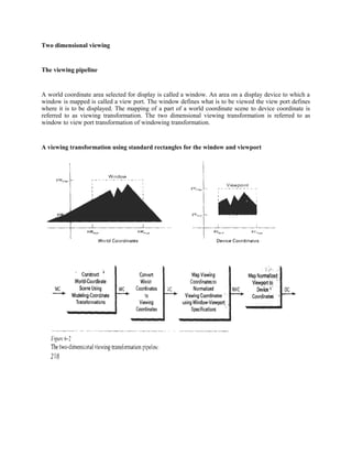
  • 1. Two dimensional viewing The viewing pipeline A world coordinate area selected for display is called a window. An area on a display device to which a window is mapped is called a view port. The window defines what is to be viewed the view port defines where it is to be displayed. The mapping of a part of a world coordinate scene to device coordinate is referred to as viewing transformation. The two dimensional viewing transformation is referred to as window to view port transformation of windowing transformation. A viewing transformation using standard rectangles for the window and viewport
  • 2. The viewing transformation in several steps, as indicated in Fig. First, we construct the scene in world coordinates using the output primitives. Next to obtain a particular orientation for the window, we can set up a two-dimensional viewing-coordinate system in the world coordinate plane, and define a window in the viewing-coordinate system. We then define a viewport in normalized coordinates (in the range from 0 to 1) and map the viewing- coordinate description of the scene to normalized coordinates. At the final step all parts of the picture that lie outside the viewport are clipped, and the contents of the viewport are transferred to device coordinates. By changing the position of the viewport, we can view objects at different positions on the display area of an output device. The viewing- coordinate reference frame is used to provide a method for setting up arbitrary orientations for rectangular windows. Once the viewing reference frame is established, we can transform descriptions in world coordinates to viewing coordinates.
  • 3. Window to view port coordinate transformation: A point at position (xw,yw) in a designated window is mapped to viewport coordinates (xv,yv) so that relative positions in the two areas are the same. The figure illustrates the window to view port mapping. A point at position (xw,yw) in the window is mapped into position (xv,yv) in the associated view port. To maintain the same relative placement in view port as in window
  • 4. The conversion is performed with the following sequence of transformations. 1. Perform a scaling transformation using point position of (xw min, yw min) that scales the window area to the size of view port. 2. Translate the scaled window area to the position of view port. Relative proportions of objects are maintained if scaling factor are the same(Sx=Sy). Otherwise world objects will be stretched or contracted in either the x or y direction when displayed on output device. For normalized coordinates, object descriptions are mapped to various display devices. Any number of output devices can be open in particular application and another window view port transformation can be performed for each open output device. This mapping called the work station transformation is accomplished by selecting a window area in normalized apace and a view port are in coordinates of display device. Mapping selected parts of a scene in normalized coordinate to different video monitors with work station transformation.
  • 5. Clipping operation Any procedure that identifies those portions of a picture that are inside or outside of a specified region of space is referred to as clipping algorithm or clipping. The region against which an object is to be clipped is called clip window. Algorithm for clipping primitive types: Point clipping Line clipping (Straight-line segment) Area clipping Curve clipping Text clipping Line and polygon clipping routines are standard components of graphics packages. Point Clipping
  • 6. Clip window is a rectangle in standard position. A point P=(x,y) for display, if following inequalities are satisfied: xwmin <= x <= xwmax ywmin <= y <= ywmax where the edges of the clip window (xwmin,xwmax,ywmin,ywmax) can be either the world- coordinate window boundaries or viewport boundaries. If any one of these four inequalities is not satisfied, the point is clipped (not saved for display). Line Clipping A line clipping procedure involves several parts. First we test a given line segment whether it lies completely inside the clipping window. If it does not we try to determine whether it lies completely outside the window . Finally if we can not identify a line as completely inside or completely outside, we perform intersection calculations with one or more clipping boundaries. Process lines through “inside-outside” tests by checking the line endpoints. A line with both endpoints inside all clipping boundaries such as line from P1 to P2 is saved. A line with both end point outside any one of the clip boundaries line P3P4 is outside the window. Line clipping against a rectangular clip window
  • 7. All other lines cross one or more clipping boundaries. For a line segment with end points (x1,y1) and (x2,y2) one or both end points outside clipping rectangle, the parametric representation X=x1 + u(x2-x1) Y= y1+u(y2-y1), 0<=u<=1 Could be used to determine values u for an intersection with the clipping boundary coordinates. If the value of u for an intersection with a rectangle boundary edge is outside the range of 0 to 1, the line does not enter the interior of the window at that boundary. If the value of u is within the range from 0 to 1, the line segment does indeed cross into the clipping area. This method can be applied to each clipping boundary edge in to determined whether any part of line segment is to displayed. Cohen-Sutherland Line Clipping This is one of the oldest and most popular line-clipping procedures. The method speeds up the processing of line segments by performing initial tests that reduce the number of intersections that must be calculated. Every line endpoint in a picture is assigned a four digit binary code called a region code that identifies the location of the point relative to the boundaries of the clipping rectangle.
  • 8. Binary region codes assigned to line end points according to relative position with respect to the clipping rectangle. Regions are set up in reference to the boundaries. Each bit position in region code is used to indicate one of four relative coordinate positions of points with respect to clip window: to the left, right, top or bottom. By numbering the bit positions in the region code as 1 through 4 from right to left, the coordinate regions are corrected with bit positions as bit 1: left bit 2: right bit 3: below bit4: above
  • 9. A value of 1 in any bit position indicates that the point is in that relative position. Otherwise the bit position is set to 0. If a point is within the clipping rectangle the region code is 0000. A point that is below and to the left of the rectangle has a region code of 0101. Bit values in the region code are determined by comparing endpoint coordinate values (x,y) to clip boundaries. Bit1 is set to 1 if x <xwmin. For programming language in which bit manipulation is possible region-code bit values can be determined with following two steps. (1) Calculate differences between endpoint coordinates and clipping boundaries. (2) Use the resultant sign bit of each difference calculation to set the corresponding value in the region code. bit 1 is the sign bit of x – xwmin bit 2 is the sign bit of xwmax - x bit 3 is the sign bit of y – ywmin bit 4 is the sign bit of ywmax - y. Once we have established region codes for all line endpoints, we can quickly determine which lines are completely inside the clip window and which are clearly outside. Any lines that are completely contained within the window boundaries have a region code of 0000 for both endpoints, and we accept these lines. Any lines that have a 1 in the same bit position in the region codes for each endpoint are completely outside the clipping rectangle, and we reject these lines. We would discard the line that has a region code of 1001 for one endpoint and a code of 0101 for the other endpoint. Both endpoints of this line are left of the clipping rectangle, as indicated by the 1 in the first bit position of each region code.
  • 10. A method that can be used to test lines for total clipping is to perform the logical and operation with both region codes. If the result is not 0000,the line is completely outside the clipping region. Lines that cannot be identified as completely inside or completely outside a clip window by these tests are checked for intersection with window boundaries. Line extending from one coordinates region to another may pass through the clip window, or they may intersect clipping boundaries without entering window. Cohen-Sutherland line clipping starting with bottom endpoint left, right , bottom and top boundaries in turn and find that this point is below the clipping rectangle. Starting with the bottom endpoint of the line from P1 to P2, we check P1 against the left, right, and bottom boundaries in turn and find that this point is below the clipping rectangle. We then find the intersection point P1 with the bottom boundary and discard the line section from P‟ 1 to P1 .‟ The line now has been reduced to the section from P1 to P‟ 2,Since P2, is outside the clip window, we check this endpoint against the boundaries and find that it is to the left of the window. Intersection point P2 is calculated, but this point is above the window. So the final intersection calculation yields P‟ 2”, and the line from P1 to P‟ 2”is saved. This completes processing for this line, so we save this part and go on to the next line. Point P3 in the next line is to the left of the clipping rectangle, so we determine the intersection P3‟, and eliminate the line section from P3 to P3'. By checking region codes for the line section from P3'to P4 we find that the remainder of the line is below the clip window and can be discarded also. Intersection points with a clipping boundary can be calculated using the slope-intercept form of the line equation. For a line with endpoint coordinates (x1,y1) and (x2,y2) and the y coordinate of the intersection point with a vertical boundary can be obtained with the calculation.
  • 11. y =y1 +m (x-x1) where x value is set either to xwmin or to xwmax and slope of line is calculated as m = (y2- y1) / (x2- x1) the intersection with a horizontal boundary the x coordinate can be calculated as x= x1 +( y- y1) / m with y set to either to ywmin or to ywmax. Liang – Barsky line Clipping: Based on analysis of parametric equation of a line segment, faster line clippers have been developed, which can be written in the form : x = x1 + u ∆x y = y1 + u ∆y 0<=u<=1 where ∆x = (x2 - x1) and ∆y = (y2 - y1) In the Liang-Barsky approach we first the point clipping condition in parametric form : xwmin <= x1 + u ∆x <=. xwmax ywmin <= y1 + u ∆y <= ywmax Each of these four inequalities can be expressed as µpk <= qk. k=1,2,3, 4
  • 12. the parameters p & q are defined as Any line that is parallel to one of the clipping boundaries have pk=0 for values of k corresponding to boundary k=1,2,3,4 correspond to left, right, bottom and top boundaries. For values of k, find qk<0, the line is completely out side the boundary. If qk >=0, the line is inside the parallel clipping boundary. When pk<0 the infinite extension of line proceeds from outside to inside of the infinite extension of this clipping boundary. If pk>0, the line proceeds from inside to outside, for non zero value of pk calculate the value of u, that corresponds to the point where the infinitely extended line intersect the extension of boundary k as u = qk / pk For each line, calculate values for parameters u1and u2 that define the part of line that lies within the clip rectangle. The value of u1 is determined by looking at the rectangle edges for which the line proceeds from outside to the inside (p<0). For these edges we calculate rk = qk / pk The value of u1 is taken as largest of set consisting of 0 and various values of r. The value of u2 is determined by examining the boundaries for which lines proceeds from inside to outside (P>0).
  • 13. A value of rkis calculated for each of these boundaries and value of u2 is the minimum of the set consisting of 1 and the calculated r values. If u1>u2, the line is completely outside the clip window and it can be rejected. Line intersection parameters are initialized to values u1=0 and u2=1. for each clipping boundary, the appropriate values for P and q are calculated and used by function Cliptest to determine whether the line can be rejected or whether the intersection parameter can be adjusted. When p<0, the parameter r is used to update u1. When p>0, the parameter r is used to update u2. If updating u1 or u2 results in u1>u2 reject the line, when p=0 and q<0, discard the line, it is parallel to and outside the boundary.If the line has not been rejected after all four value of p and q have been tested , the end points of clipped lines are determined from values of u1 and u2. The Liang-Barsky algorithm is more efficient than the Cohen-Sutherland algorithm since intersections calculations are reduced. Each update of parameters u1 and u2 require only one division and window intersections of these lines are computed only once. Cohen-Sutherland algorithm, can repeatedly calculate intersections along a line path, even through line may be completely outside the clip window. Each intersection calculations require both a division and a multiplication. Text clipping There are several techniques that can be used to provide text clipping in a graphics package. The clipping technique used will depend on the methods used to generate characters and the requirements of a particular application.
  • 14. The simplest method for processing character strings relative to a window boundary is to use the all-or-none string-clipping strategy shown in Fig. . If all of the string is inside a clip window, we keep it. Otherwise, the string is discarded. This procedure is implemented by considering a bounding rectangle around the text pattern. The boundary positions of the rectangle are then compared to the window boundaries, and the string is rejected if there is any overlap. This method produces the fastest text clipping. Text clipping using a bounding rectangle about the entire string An alternative to rejecting an entire character string that overlaps a window boundary is to use the all-or-none character-clipping strategy. Here we discard only those characters that are not completely inside the window .In this case, the boundary limits of individual characters are compared to the window. Any character that either overlaps or is outside a window boundary is clipped. Text clipping using a bounding rectangle about individual characters. A final method for handling text clipping is to clip the components of individual characters. We now treat characters in much the same way that we treated lines. If an individual character overlaps a clip window boundary, we clip off the parts of the character that are outside the window. Text Clipping performed on the components of individual characters