huhg h7gf

1. Different cases for Line Clipping
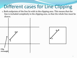
1. Both endpoints of the line lie with in the clipping area. This means that the
line is included completely in the clipping area, so that the whole line must be
drawn.
Clip
rectangle
B
A
B
A
1

2. Conti….
3. Both end points are located outside the clipping area and the line do not intersect the
clipping area. In the case , the line lies completely outside the clipping area and can be
neglected for the scene.
4. Both endpoints are located outside the clipping area and the line intersect the clipping
area. The two intersection points of the line with the clipping are must be determined.
Only the part of the line between these two intersection points should be drawn.
C
D’
B
A
G’
H'
Clip
rectangle
B
A
D
D’
C
G’
H'
G
H
I’
I
J’
J
E
F
2

3. COHEN-SUTHERLAND LINE CLIPPING
ALGORITHM
 This algorithm divides a 2D space into 9parts,of which only the middle part is
visible.
 Cohen- Sutherland subdivision line clipping algorithm was developed by Dan
Cohen and lvan Sutherland. This method is used:
i. To save a line segment.
ii. To discard line segment or,
iii. To divide the line according to window co- ordinate.
 Cohen Sutherland performs line clipping in two phases:
Phase1: Find visibility of line.
Phase2: clip the line falling in category 3 (candidate for Clipping).
3

4. COHEN-SUTHERLAND LINE
CLIPPING ALGORITHM
 Every line end point in a picture is assigned a four bit binary code, called a region
code, that identify the location of the point relative to the boundaries of the
clipping rectangle. Region are set up in reference as shown in figure:
Figure :Bit Code for Cohen- Sutherland clipping
window
ywmax
ywmin
xwmin xwmax
y
LEFT RIGHT
TOP
BOTTOM
x
1001
0001
0101
1000
0010
0100
1010
0110
0000
4

5. COHEN-SUTHERLAND LINE
CLIPPING ALGORITHM
Every bit position in the region code is used to indicate one of the four relative
coordinate position of the point with respect to the clip window: to the Left, Right ,
Top or Bottom. By numbering the bit position in the region code as 1 through 4 from
right to left, the coordinate region can be correlated with the bit position as . This rule
is also called TBRL code(Top-Bottom-Right-Left).
5

6. COHEN-SUTHERLAND LINE
CLIPPING ALGORITHM
Following rules are used for clipping by Cohen-Sutherland line clipping algorithm:
Visible : Any lines that are completely contained within the window boundaries have a
region code of 0000 for both endpoints, and we trivially accept these lines . For example,
Line segment P1P2 is visible in the figure.
Invisible : Any lines that have a 1 in the same bit position in the region code for each
endpoints are completely outside the clipping rectangle and the line segment is invisible ,
Ad we trivially reject these lines. We would discard the line that has a region code of 0001
For one endpoint and a code of 0101 for the other endpoint. Both end points of the line are
Left of the clipping rectangle , as indicated by the 1 in the first position of each region code.
6

7. Cont…….
window
ywmax
ywmin
xwmin xwmax
y
LEFT RIGHT
TOP
BOTTOM
x
1001
0001
0101
1000
0010
0100
1010
0110
P8
P7
0000
P1
P2
P3
P4
P6
P5
Figure :Cohen- Sutherland clipping techniques
Clipping Candidate or indeterminate : A line segment is said to be indeterminate
If the bitwise logical AND of the region codes of the end points is equal to(0000).
For example: line segment P3P4 having endpoint codes(0100) and (0010) and P7P8 having endpoints
Codes (0010) and (1000) in the figure. These line segments may or may not process the window
Boundaries as line segment P7P8 is invisible but line segment P3P4 is partially visible and must be
Clipped.
7

8. COHEN-SUTHERLAND LINE
CLIPPING ALGORITHM
Advantage and Disadvantages:
 Will do unnecessary clipping.
 Not the most efficient.
 Clipping and testing are done in fixed order.
 Easy to program.
 Efficient when most of lines to be clipped are either rejected or
accepted.
8

9. Intersection, Calculation and
Clipping
 Line that can not be identified as completely inside a clip window by
these test are checked for intersection with the window boundaries.We
begin the clipping process for a line by comparing an outside endpoint
to a window boundary to determine how much of the line can be
discard . Then the remaining part of the line is checked against the
other boundaries,and we continue until either the line is totally discard
or a section is found inside the window.We set up our algorithm to
check line endpoints against clipping boundaries in the order
left,right,bottom,top.
 TO ilustrate the specific step in clipping line against rectangular
boundary using the Cohen-Suterland algorithm,We show the linein
figure could be processed.
9

10.  Starting with the bottom endpoints of the line from p1 to p2, we check p1
against the left right bottom boundaries in turn and find that this point is
below the window. We then find the intersection point p1’ with the window
boundary and discard the line section from p1 to p1’.The line now be reduced to
the section from p1’ to p2.
 Since P2 is outside the clip window. We check these end points against the
boundary. find that it is to the left of the window. Intersection point p2’ is
calculated . But this point is outside the window. So the final intersection
calculation is p2” and the line from P1’ to p2” is saved. This complete
processing for these line . So we save this part and go on to the next line.
 Point P3 is the next line is to the left of the clipping window, so we
determine the intersection point P3 and eliminate the line from P3 to P3’.By
checking region code for the line section from P3’ to P4. We find the remainder
of the line is below the clip window and can be discarded also.
Intersection Calculation and Clipping
10

11. Intersection Calculation and Clipping
window
xwmin xwmax
y
TOP
BOTTOM
x
1001
0001
0101
1000
0010
0100
1010
0110
0000
ywmax
ywmin
LEFT RIGHT
P2
P2’
P2”
P1’
P1
P3’
P3
P4
Figure : lines extending from one coordinate region to another may pass through the
Clip window, or they may intersect clipping boundaries without entering the window.
11

12. Intersection and calculation
clipping
 Q.Intersection point with a clipping boundary can be
calculated using the slope intersect for the line of
equation.
 X min=2,X max=8, y min=2 y max=8
 EF:E(3,10) & F(6,12)
 GH:G(4,1) &H (10,6)
Formula:
 M=Y2-Y1/X2-X1
 Xi=X1+1/m(Yi-Y1)
 Where the x value is set to either Xmin or to a x max
 Yi=Y1+m(Xi-X1)
12

13. Mid point subdivision algorithm
 This method divide the line into three category:
I. Category 1: Visible line
II. Category 2: not visible line
III. Category 3: candidate for Clipping.
An alternative way to process a line in category 3 is based on binary
search.The line is divided at its midpointsinto two shorter line segments.
Each line in a category three is divided again into shorter segments and
categorized.This bisection and categorization process continue until eavh
line segment that spans across a window boundary reaches a threshold for
line size and all other segments are either in a category 1 (visible) or in
category 2 (Not visible.)
13

14. Mid-point subdivision algorithm
The mid points coordinates are (x m, y m) of a line joining the points(X1,Y1)and (X2,Y2)
are given by:
X m= X1+X2/2 and
Y M= Y1+Y2/2 Q
P
6
7
8
5
1
I1
I2
2
4
3
Figure: illustrates how midpoint subdivision is used to zoom in onto the two Intersection points I1 and I2 with 10 bisection.
14

15. Comparison b/w Cohen-Sutherland and Mid-point subdivision clipping Algorithm
• Midpoint subdivision algorithm is a special case of Cohen-sutherland algorithm,
where the intersection is not computed by equation solving. It is computed by a
midpoint approximation method, which is suitable for hardware and it is very
fast and efficient.
• The maximum time is consume in the clipping process is to do intersection calculation
with the window boundaries.
• The Cohen-sutherland algorithm reduces these calculation by first discarding that lines
those can be trivially accepted or rejected.
15

16. Polygon Clipping
 The simplest curve is a line segment or simply a line. A sequence of line where the
following line starts where the previous one ends is called a polyline. If the last line
segment of the polyline ends where the first line segment started, the polyline is called
a polygon. A polygon is defined by n number of sides in the polygon. We can divide
polygon into two classes.
 A convex polygon is a polygon such that for any two points inside the polygon , all
the point of the line segment connecting them are also inside the polygon. A triangle
is always a convex one.
Polygon
Convex
Polygon
Concave
Polygon
P
Q
16

17. Conti…
 A Concave polygon is one which is not convex.. A polygon is said to be a concave
if the line joining any two interior points of the polygon does not lies completely
inside the polygon.
 There are four possible cases when processes vertices in sequence around the
parameter of the polygon. As each pair of adjacent polygon vertices is passed to a
window boundary clipper. We make the following test.
P
Q
17

18. Conti…
 Case 1: If the first vertex is outside the window boundary and second vertex
is inside the window boundary then both the intersection point of a polygon
edge with the window boundary and second vertex are added to the output
vertex list.
 Case 2: If both input vertices are inside the window boundary. Only the
second vertex is added to the Vertex list
Case3: If the first vertex is inside the window boundary and the second
vertex is outside the window boundary then only the edge intersection with the
window boundary is added to the output vertex list.
 Case 4: If both the input vertices are outside the window boundary then
nothing is save to the output list.
18

19. SUTHERLAND AND HODGEMAN
ALGORITHM(Polygon clipping)
 Polygon clipping is a process of clipping a polygon by considering
the edge of that as different line segments. If a polygon is clipped
against a rectangular window then it is possible that we get various
unconnected edges of a polygon. To get a closed polygon of unconnected
edges we connect theses edges along the side of a clipping window to
form a closed polygon.
 The Sutherland –Hodgeman polygon clipping algorithm clips polygon
against convex clipping windows. The Sutherland Hodgeman Polygon
clipping algorithm may produce connecting lines that were not in the
original polygon. When the subject polygon is concave theses connecting
lines may be undesirable artifacts.
 There are four situation to save vertices in output vertex list.
19

20. Conti……
1. If the first vertex is outside the window boundary and second vertex is inside the
window boundary then both the intersection point of a polygon edge with the
window boundary and second vertex are added to the output vertex list.Ex:save v1’,v2.
POLYGON
WINDOW(W)
2. If both input vertices are inside the window boundary. Only the second vertex is
added to the Vertex list
POLYGON
WINDOW(w)
V1
V1’
V2
V1
V2
20

21. Cont…..
3. If the first vertex is inside the window boundary and the second vertex is
outside the window boundary then only the edge intersection with the
window boundary is added to the output vertex list.Ex: v1’, v1.
POLYGON
WINDOW(W)
4. If both the input vertices are outside the window boundary then nothing is
save to the output list.
POLYGON
WINDOW(W)
’
V2
V1
V2
V1’
V1
21