easy maths formula

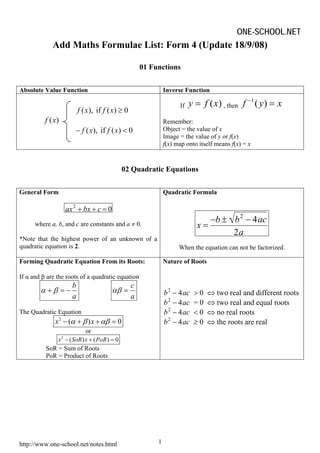
1. ONE-SCHOOL.NET
http://www.one-school.net/notes.html 1
Add Maths Formulae List: Form 4 (Update 18/9/08)
01 Functions
Absolute Value Function Inverse Function
If ( )y f x= , then
1
( )f y x−
=
Remember:
Object = the value of x
Image = the value of y or f(x)
f(x) map onto itself means f(x) = x
02 Quadratic Equations
General Form
ax2
+ bx + c = 0
where a, b, and c are constants and a ≠ 0.
*Note that the highest power of an unknown of a
quadratic equation is 2.
Quadratic Formula
x =
−b ± b2
− 4ac
2a
When the equation can not be factorized.
Forming Quadratic Equation From its Roots:
If α and β are the roots of a quadratic equation
b
a
α β+ = −
c
a
αβ =
The Quadratic Equation
2
( ) 0x xα β αβ− + + =
or
2
( ) ( ) 0x SoR x PoR− + =
SoR = Sum of Roots
PoR = Product of Roots
Nature of Roots
b2
− 4ac > 0 ⇔ two real and different roots
b2
− 4ac = 0 ⇔ two real and equal roots
b2
− 4ac < 0 ⇔ no real roots
b2
− 4ac ≥ 0 ⇔ the roots are real
( )f x
( ), if ( ) 0f x f x ≥
( ), if ( ) 0f x f x− <

2. ONE-SCHOOL.NET
http://www.one-school.net/notes.html 2
03 Quadratic Functions
General Form
2
( )f x ax bx c= + +
where a, b, and c are constants and a ≠ 0.
*Note that the highest power of an unknown of a
quadratic function is 2.
0a > ⇒ minimum ⇒ ∪ (smiling face)
0a < ⇒ maximum ⇒ ∩ (sad face)
Completing the square:
2
( ) ( )f x a x p q= + +
(i) the value of x, x p= −
(ii) min./max. value = q
(iii) min./max. point = ( , )p q−
(iv) equation of axis of symmetry, x p= −
Alternative method:
2
( )f x ax bx c= + +
(i) the value of x,
2
b
x
a
= −
(ii) min./max. value = ( )
2
b
f
a
−
(iii) equation of axis of symmetry,
2
b
x
a
= −
Quadratic Inequalities
0a > and ( ) 0f x > 0a > and ( ) 0f x <
orx a x b< > a x b< <
Nature of Roots
2
4 0b ac− > ⇔ intersects two different points
at x-axis
2
4 0b ac− = ⇔ touch one point at x-axis
2
4 0b ac− < ⇔ does not meet x-axis
04 Simultaneous Equations
To find the intersection point ⇒ solves simultaneous equation.
Remember: substitute linear equation into non- linear equation.
ba ba

3. ONE-SCHOOL.NET
http://www.one-school.net/notes.html 3
05 Indices and Logarithm
Fundamental if Indices
Zero Index, 0
1a =
Negative Index, 1 1
a
a−
=
1
( )
a b
b a
−
=
Fractional Index
1
nn aa =
n m
m
n aa =
Laws of Indices
m n m n
a aa +
× =
m n m n
a aa −
÷ =
( )m n m n
a a ×
=
( )n n n
ab a b=
( )
n
n
n
a a
b b
=
Fundamental of Logarithm
log x
a y x a y= ⇔ =
log 1a a =
log x
a a x=
log 1 0a =
Law of Logarithm
log log loga a amn m n= +
log log loga a a
m
m n
n
= −
log a mn
= n log a m
Changing the Base
log
log
log
c
a
c
b
b
a
=
1
log
loga
b
b
a
=

4. ONE-SCHOOL.NET
http://www.one-school.net/notes.html 4
06 Coordinate Geometry
Distance and Gradient
Distance Between Point A and C =
( ) ( )2
21
2
21 xxxx −+−
Gradient of line AC, 2 1
2 1
y y
m
x x
−
=
−
Or
Gradient of a line,
int
int
y ercept
m
x ercept
⎛ ⎞−
= −⎜ ⎟
−⎝ ⎠
Parallel Lines Perpendicular Lines
When 2 lines are parallel,
21 mm = .
When 2 lines are perpendicular to each other,
1 2 1m m× = −
m1 = gradient of line 1
m2 = gradient of line 2
Midpoint A point dividing a segment of a line
Midpoint, 1 2 1 2
,
2 2
x x y y
M
+ +⎛ ⎞
= ⎜ ⎟
⎝ ⎠
A point dividing a segment of a line
1 2 1 2
,
nx mx ny my
P
m n m n
+ +⎛ ⎞
=⎜ ⎟
+ +⎝ ⎠

5. ONE-SCHOOL.NET
http://www.one-school.net/notes.html 5
Area of triangle:
Area of Triangle
=
2
1
( ) ( )31 2 2 3 1 2 1 3 2 1 3
1
2
A x y x y x y x y x y x y= + + − + +
Equation of Straight Line
Gradient (m) and 1 point (x1, y1)
given
1 1( )y y m x x− = −
2 points, (x1, y1) and (x2, y2) given
1 2 1
1 2 1
y y y y
x x x x
− −
=
− −
x-intercept and y-intercept given
1
x y
a b
+ =
Equation of perpendicular bisector ⇒ gets midpoint and gradient of perpendicular line.
Form of Equation of Straight Line
General form Gradient form Intercept form
0ax by c+ + = y mx c= +
m = gradient
c = y-intercept
1
x y
a b
+ =
a = x-intercept
b = y-intercept
Information in a rhombus:
(i) same length ⇒ AB BC CD AD= = =
(ii) parallel lines ⇒ AB CDm m= or AD BCm m=
(iii) diagonals (perpendicular) ⇒ 1AC BDm m× = −
(iv) share same midpoint ⇒ midpoint AC = midpoint
BD
(v) any point ⇒ solve the simultaneous equations
b
m
a
= −
A B
C
D

6. ONE-SCHOOL.NET
http://www.one-school.net/notes.html 6
Equation of Locus
( use the formula of
distance)
The equation of the locus of a
moving point ),( yxP which
is always at a constant
distance (r) from a fixed point
A ),( 11 yx is
PA r=
22
1
2
1 )()( ryyxx =−+−
The equation of the locus of a
moving point ),( yxP which is
always at a constant distance
from two fixed points
A ),( 11 yx and B ),( 22 yx with
a ratio nm: is
PA m
PB n
=
2
2
2
22
2
1
2
1
)()(
)()(
n
m
yyxx
yyxx
=
−+−
−+−
The equation of the locus of a moving
point ),( yxP which is always
equidistant from two fixed points A and B
is the perpendicular bisector of the
straight line AB.
PA PB=
2 2 2 2
1 1 2 2( ) ( ) ( ) ( )x x y y x x y y− + − = − + −
Remember:
y-intercept ⇒ 0x =
cut y-axis ⇒ 0x =
x-intercept ⇒ 0y =
cut x-axis ⇒ 0y =
**point lies on the line ⇒ satisfy the equation ⇒ substitute the value of x and of y of the point into the
equation.
More Formulae and Equation List:
SPM Form 4 Physics - Formulae List
SPM Form 5 Physics - Formulae List
SPM Form 4 Chemistry - List of Chemical Reactions
SPM Form 5 Chemistry - List of Chemical Reactions
All at One-School.net

7. ONE-SCHOOL.NET
http://www.one-school.net/notes.html 7
07 Statistics
Measure of Central Tendency
Grouped Data
Ungrouped Data
Without Class Interval With Class Interval
Mean
N
x
x
Σ
=
meanx =
sum ofx xΣ =
value of the datax =
N = total number of the
data
f
fx
x
Σ
Σ
=
meanx =
sum ofx xΣ =
frequencyf =
value of the datax =
f
fx
x
Σ
Σ
=
meanx =
frequencyf =
class mark
(lower limit+upper limit)
=
2
x =
Median
1
2
Nm T +=
When N is an odd number.
1
2 2
2
N NT T
m
+
+
=
When N is an even
number.
1
2
Nm T +=
When N is an odd number.
1
2 2
2
N NT T
m
+
+
=
When N is an even number.
C
f
FN
Lm
m
⎟⎟
⎠
⎞
⎜⎜
⎝
⎛ −
+= 2
1
m = median
L = Lower boundary of median class
N = Number of data
F = Total frequency before median class
fm = Total frequency in median class
c = Size class
= (Upper boundary – lower boundary)
Measure of Dispersion
Grouped Data
Ungrouped Data
Without Class Interval With Class Interval
variance 2
2
2
x
N
x
−=
∑σ
2
2
2
x
f
fx
−=
∑
∑σ
2
2
2
x
f
fx
−=
∑
∑σ
Standard
Deviation
variance=σ
( )
2
x x
N
σ
Σ −
=
2
2x
x
N
σ
Σ
= −
variance=σ
( )
2
x x
N
σ
Σ −
=
2
2x
x
N
σ
Σ
= −
variance=σ
( )
2
f x x
f
σ
Σ −
=
Σ
2
2fx
x
f
σ
Σ
= −
Σ

8. ONE-SCHOOL.NET
http://www.one-school.net/notes.html 8
Effects of data changes on Measures of Central Tendency and Measures of dispersion
08 Circular Measures
Terminology
Convert degree to radian:
Convert radian to degree:
180
π
×
radians degrees
180
π
×
( )radians
180
o
x x
π
= ×
180
radians ( )degreesx x
π
= ×
Remember:
180 radπ=
360 2 radπ=
Data are changed uniformly with
+ k k− × k ÷ k
Measures of
Central Tendency
Mean, median, mode + k k− × k ÷ k
Range , Interquartile Range No changes × k ÷ k
Standard Deviation No changes × k ÷ k
Measures of
dispersion
Variance No changes × k2
÷ k2
The variance is a measure of the mean for the square of the deviations from the mean.
The standard deviation refers to the square root for the variance.
0.7 rad
???
O
1.2 rad
???

9. ONE-SCHOOL.NET
http://www.one-school.net/notes.html 9
Length and Area
r = radius
A = area
s = arc length
θ = angle
l = length of chord
Arc Length:
s rθ=
Length of chord:
2 sin
2
l r
θ
=
Area of Sector:
21
2
A r θ=
Area of Triangle:
21
sin
2
A r θ=
Area of Segment:
21
( sin )
2
A r θ θ= −
09 Differentiation
Differentiation of Algebraic Function
Differentiation of a Constant
Differentiation of a Function I
Differentiation of a Function II
1 1 0
y ax
dy
ax ax a
dx
−
=
= = =
Example
3
3
y x
dy
dx
=
=
1
n
n
y x
dy
nx
dx
−
=
=
Example
3
2
3
y x
dy
x
dx
=
=
is a constant
0
y a a
dy
dx
=
=
Example
2
0
y
dy
dx
=
=
Gradient of a tangent of a line (curve or
straight)
0
lim( )
x
dy y
dx xδ
δ
δ→
=

10. ONE-SCHOOL.NET
http://www.one-school.net/notes.html 10
Differentiation of a Function III
Differentiation of a Fractional Function
Law of Differentiation
Sum and Difference Rule
Chain Rule
and are functions inn
y u u v x
dy dy du
dx du dx
=
= ×
Example
2 5
2
5 4
4
2 4 2 4
(2 3)
2 3, therefore 4
, therefore 5
5 4
5(2 3) 4 20 (2 3)
y x
du
u x x
dx
dy
y u u
du
dy dy du
dx du dx
u x
x x x x
= +
= + =
= =
= ×
= ×
= + × = +
Or differentiate directly
1
( )
. .( )
n
n
y ax b
dy
n a ax b
dx
−
= +
= +
2 5
2 4 2 4
(2 3)
5(2 3) 4 20 (2 3)
y x
dy
x x x x
dx
= +
= + × = +
and are functions iny u v u v x
dy du dv
dx dx dx
= ±
= ±
Example
3 2
2 2
2 5
2(3) 5(2) 6 10
y x x
dy
x x x x
dx
= +
= + = +
1
1
1
Rewrite
n
n
n
n
y
x
y x
dy n
nx
dx x
−
− −
+
=
=
−
= − =
Example
1
2
2
1
1
1
y
x
y x
dy
x
dx x
−
−
=
=
−
= − =
1
n
n
y ax
dy
anx
dx
−
=
=
Example
3
2 2
2
2(3) 6
y x
dy
x x
dx
=
= =

11. ONE-SCHOOL.NET
http://www.one-school.net/notes.html 11
Product Rule Quotient Rule
2
and are functions in
u
y u v x
v
du dv
v u
dy dx dx
dx v
=
−
=
Example
2
2
2
2
2
2 2 2
2 2
2 1
2 1
2 2
(2 1)(2 ) (2)
(2 1)
4 2 2 2 2
=
(2 1) (2 1)
x
y
x
u x v x
du dv
x
dx dx
du dv
v u
dy dx dx
dx v
dy x x x
dx x
x x x x x
x x
=
+
= = +
= =
−
=
+ −
=
+
+ − +
=
+ +
Or differentiate directly
2
2
2
2 2 2
2 2
2 1
(2 1)(2 ) (2)
(2 1)
4 2 2 2 2
=
(2 1) (2 1)
x
y
x
dy x x x
dx x
x x x x x
x x
=
+
+ −
=
+
+ − +
=
+ +
and are functions iny uv u v x
dy du dv
v u
dx dx dx
=
= +
Example
3 2
3 2
2
3 2 2
(2 3)(3 2 )
2 3 3 2
2 9 4 1
=(3 2 )(2) (2 3)(9 4 1)
y x x x x
u x v x x x
du dv
x x
dx dx
dy du dv
v u
dx dx dx
x x x x x x
= + − −
= + = − −
= = − −
= +
− − + + − −
Or differentiate directly
3 2
3 2 2
(2 3)(3 2 )
(3 2 )(2) (2 3)(9 4 1)
y x x x x
dy
x x x x x x
dx
= + − −
= − − + + − −

12. ONE-SCHOOL.NET
http://www.one-school.net/notes.html 12
Gradients of tangents, Equation of tangent and Normal
If A(x1, y1) is a point on a line y = f(x), the gradient
of the line (for a straight line) or the gradient of the
tangent of the line (for a curve) is the value of
dy
dx
when x = x1.
Gradient of tangent at A(x1, y1):
gradient of tangent
dy
dx
=
Equation of tangent: 1 1( )y y m x x− = −
Gradient of normal at A(x1, y1):
normal
tangent
1
m
m
= −
1
gradient of normal
dy
dx
=
−
Equation of normal : 1 1( )y y m x x− = −
Maximum and Minimum Point
Turning point ⇒ 0
dy
dx
=
At maximum point,
0
dy
dx
=
2
2
0
d y
dx
<
At minimum point ,
0
dy
dx
=
2
2
0
d y
dx
>

13. ONE-SCHOOL.NET
http://www.one-school.net/notes.html 13
Rates of Change Small Changes and Approximation
Chain rule
dA dA dr
dt dr dt
= ×
If x changes at the rate of 5 cms -1
⇒ 5
dx
dt
=
Decreases/leaks/reduces ⇒ NEGATIVES values!!!
Small Change:
y dy dy
y x
x dx dx
δ
δ δ
δ
≈ ⇒ ≈ ×
Approximation:
new original
original
y y y
dy
y x
dx
δ
δ
= +
= + ×
small changes in
small changes in
x x
y y
δ
δ
=
=
If x becomes smaller ⇒ x NEGATIVEδ =

14. ONE-SCHOOL.NET
http://www.one-school.net/notes.html 14
10 Solution of Triangle
Sine Rule:
C
c
B
b
A
a
sinsinsin
==
Use, when given
2 sides and 1 non included
angle
2 angles and 1 side
Cosine Rule:
a2
= b2
+ c2
– 2bc cosA
b2
= a2
+ c2
– 2ac cosB
c2
= a2
+ b2
– 2ab cosC
bc
acb
A
2
cos
222
−+
=
Use, when given
2 sides and 1 included angle
3 sides
Area of triangle:
1
sin
2
A a b C=
C is the included angle of sides a
and b.
A
Ba
180 – (A+B)
a
b
A
b
A
a
b
ca
C
a
b

15. ONE-SCHOOL.NET
http://www.one-school.net/notes.html 15
Case of AMBIGUITY If ∠C, the length AC and length AB remain unchanged,
the point B can also be at point B′ where ∠ABC = acute
and ∠A B′ C = obtuse.
If ∠ABC = θ, thus ∠AB′C = 180 – θ .
Remember : sinθ = sin (180° – θ)
Case 1: When sina b A<
CB is too short to reach the side opposite to C.
Outcome:
No solution
Case 2: When sina b A=
CB just touch the side opposite to C
Outcome:
1 solution
Case 3: When sina b A> but a < b.
CB cuts the side opposite to C at 2 points
Outcome:
2 solution
Case 4: When sina b A> and a > b.
CB cuts the side opposite to C at 1 points
Outcome:
1 solution
Useful information:
In a right angled triangle, you may use the following to solve the
problems.
a
b
c
θ
(i) Phythagoras Theorem: 2 2
c a b= +
(ii)
Trigonometry ratio:
sin , cos , tanb a b
c c a
θ θ θ= = =
(iii) Area = ½ (base)(height)
C BB′
θ
180 - θ
A

16. ONE-SCHOOL.NET
http://www.one-school.net/notes.html 16
11 Index Number
Price Index Composite index
1
0
100
P
I
P
= ×
Price indexI = / Index number
P0 = Price at the base time
P1 = Price at a specific time
i
ii
W
IW
I
Σ
Σ
=
Composite IndexI =
WeightageW =
Price indexI =
, , , 100A B B C A CI I I× = ×