1. Supporting economics in higher education
Economics
Network
Maths for
Economics
PRINCIPLES AND FORMULAE
y=ex
x
1
–1 1
y=e–x
x
1
–1 1
y=ex
x
1
–1 1
y=e–x
x
1
–1 1
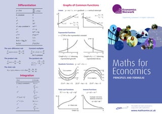
Exponential functions
e ≈ 2.7183 is the exponential constant
Graph of y = ex showing
exponential growth
Graph of y = e–x showing
exponential decay
if a is positive
x
–b / 2a
(1)
(2)
(3)
if a is negative
x
–b / 2a
(3)
(2)
(1)
if a is positive
x
–b / 2a
(1)
(2)
(3)
if a is negative
x
–b / 2a
(3)
(2)
(1)
Quadratic functions y = ax2 + bx + c
TC
Output (q)
a
a = fixed cost
TC
Output (q)
a
a = fixed cost
y
x
Example: Unit price
elasticity of demand
Total cost functions
TC = a + bq – cq2 + dq3
Inverse functions
y = a/x = ax–1
q = a/p = ap–1
(1) b2 – 4ac < 0; (2) b2 – 4ac = 0; (3) b2 – 4ac > 0
Differentiation Graphs of Common Functions
Integration
The sum–difference rule Constant multiples
The product rule The quotient rule
The chain rule
x
v
x
u
x
v
x
u
x d
d
d
d
))
(
)
(
(
d
d
±
=
±
x
f
k
x
f
k
x d
d
))
(
(
d
d
=
x
u
v
x
v
u
uv
x d
d
d
d
)
(
d
d
+
=
2
d
d
d
d
d
d
v
x
v
u
x
u
v
v
u
x
–
=
x
u
u
y
x
y
x
u
u
u
y
y
d
d
d
d
d
d
then
,
)
(
where
,
)
(
If .
=
=
=
x
v
x
u
x
v
x
u
x d
d
d
d
))
(
)
(
(
d
d
±
=
±
x
f
k
x
f
k
x d
d
))
(
(
d
d
=
x
u
v
x
v
u
uv
x d
d
d
d
)
(
d
d
+
=
2
d
d
d
d
d
d
v
x
v
u
x
u
v
v
u
x
–
=
x
u
u
y
x
y
x
u
u
u
y
y
d
d
d
d
d
d
then
,
)
(
where
,
)
(
If .
=
=
=
x
v
x
u
x
v
x
u
x d
d
d
d
))
(
)
(
(
d
d
±
=
±
x
f
k
x
f
k
x d
d
))
(
(
d
d
=
x
u
v
x
v
u
uv
x d
d
d
d
)
(
d
d
+
=
2
d
d
d
d
d
d
v
x
v
u
x
u
v
v
u
x
–
=
x
u
u
y
x
y
x
u
u
u
y
y
d
d
d
d
d
d
then
,
)
(
where
,
)
(
If .
=
=
=
x
v
x
u
x
v
x
u
x d
d
d
d
))
(
)
(
(
d
d
±
=
±
x
f
k
x
f
k
x d
d
))
(
(
d
d
=
x
u
v
x
v
u
uv
x d
d
d
d
)
(
d
d
+
=
2
d
d
d
d
d
d
v
x
v
u
x
u
v
v
u
x
–
=
x
u
u
y
x
y
x
u
u
u
y
y
d
d
d
d
d
d
then
,
)
(
where
,
)
(
If .
=
=
=
∫ x
x
f d
)
(
x
x
f )
(
c
x
+
c
+
2
2
c
x
+
3
3
x2
ex
ekx
x , (n = –1)
n
c
x
x
+
n+1
n+1
c
k
k
k, (any) constant c
ekx
+
c
+
ex
ln x + c
x = 1/x
–1
x
v
x
u
x
v
x
u
x d
d
d
d
))
(
)
(
(
d
d
±
=
±
x
f
k
x
f
k
x d
d
))
(
(
d
d
=
x
u
v
x
v
u
uv
x d
d
d
d
)
(
d
d
+
=
2
d
d
d
d
d
d
v
x
v
u
x
u
v
v
u
x
–
=
x
u
u
y
x
y
x
u
u
u
y
y
d
d
d
d
d
d
then
,
)
(
where
,
)
(
If .
=
=
=
y
x
Positive gradient
c (x1, y1)
(x2, y2)
1
2
1
2
x
x
y
y
m
–
–
=
y
x
Negative gradient
c (x1, y1)
(x2, y2)
1
2
1
2
x
x
y
y
m
–
–
=
x
Positi
c (x1, y1)
1
2
1
2
x
x
y
y
m
–
–
=
y
x
Negative gradient
c (x1, y1)
(x2, y2)
1
2
1
2
x
x
y
y
m
–
–
=
Linear y = mx + c; m = gradient; c = vertical intercept
y = f(x)
k, constant 0
x 1
x2 2x
x3 3x2
xn, any constant n nxn–1
ex ex = y
ekx kekx = ky
e f(x) f’(x)e f(x)
ln x 1/x
ln kx = logekx 1/x
ln f(x) f’(x)/f(x)
dy
dx
= f’(x)
for k constant
www.mathcentre.ac.uk
This leaflet has been produced in
conjunction with mathcentre
2. Arithmetic Algebra
Proportion and Percentage
When multiplying or dividing positive and negative
numbers, the sign of the result is given by:
+ and + gives + e.g. 6 x 3 = 18; 21 ÷ 7 = 3
– and + gives – e.g. (–6) x 3 = –18 (–21) ÷ 7 = –3
+ and – gives – e.g. 6 x (–3) = –18 21 ÷ (–7) = –3
– and – gives + e.g. (–6) x (–3) = 18 (–21) ÷ (–7) = 3
Order of calculation
First: brackets
Second: x and ÷
Third: + and –
Fractions
Fraction =
Adding and subtracting fractions
To add or subtract two fractions, first rewrite each fraction
so that they have the same denominator. Then, the
numerators are added or subtracted as appropriate and
the result is divided by the common denominator: e.g.
Multiplying fractions
To multiply two fractions, multiply their numerators and
then multiply their denominators: e.g.
Dividing fractions
To divide two fractions, invert the second and then
multiply: e.g.
Series (e.g. for discounting)
1 + x + x2 + x3 + x4 + … = 1/(1–x)
1 + x + x2 + x3 + … + xk = (1–xk+1)/(1–x)
(where 0 < x < 1)
numerator
denominator
20
31
=
20
15
+
20
16
=
4
3
+
5
4
77
15
=
11
5
7
3
10
9
=
2
3
5
3
=
3
2
÷
5
3
20
31
=
20
15
+
20
16
=
4
3
+
5
4
77
15
=
11
5
7
3
10
9
=
2
3
5
3
=
3
2
÷
5
3
20
31
=
20
15
+
20
16
=
4
3
+
5
4
77
15
=
11
5
7
3
10
9
=
2
3
5
3
=
3
2
÷
5
3
Removing brackets
a(b + c) = ab + ac a(b – c) = ab – ac
(a + b)(c + d) = ac + ad + bc + bd
(a + b)2 = a2 + b2 + 2ab; (a - b)2 = a2 + b2 – 2ab
(a + b)(a – b) = a2 – b2
Formula for solving a quadratic equation
Laws of indices
Laws of logarithms
y = logbx means by = x and b is called the base
e.g. log10 2 = 0.3010 means 100.3010 = 2.000 to 4 sig figures
Logarithms to base e, denoted loge, or alternatively ln,
are called natural logarithms. The letter e stands for the
exponential constant, which is approximately 2.7183.
a
ac
b
b
x
2
4
2
–
±
–
=
If ax2 + bx + c = 0, then
n
m
n
m
a
a
a +
= n
m
n
m
a
a
a –
= mn
n
m
a
a =
)
(
1
0
=
a m
m
a
a
1
=
– n
n
a
a =
/
1 m
n
n
a
a =
/
m
B
A
AB ln
ln
ln +
= B
A
B
A
ln
ln
ln –
= A
n
An
ln
ln =
; ;
%
5
.
62
100
8
5
is
percentage
a
as
8
5
=
%
10
=
10
1
%
25
=
4
1
%
50
=
2
1
%
75
=
4
3
%
5
.
62
100
8
5
is
percentage
a
as
8
5
=
%
10
=
10
1
%
25
=
4
1
%
50
=
2
1
%
75
=
4
3
To convert a fraction into a percentage, multiply by 100
and express the result as a percentage. An example is:
Ratios are simply an alternative way of expressing
fractions. Consider dividing £200 between two people in
the ratio of 3:2. This means that for every £3 the first person
gets, the second person gets £2. So the first gets 3/5 of the
total (i.e. £120) and the second gets 2/5 (i.e. £80).
Generally, to split a quantity in the ratio m : n, the quantity
is divided into m/(m + n) and n/(m + n) of the total.
Some common conversions are
Sigma Notation
The Greek Alphabet
The Greek capital letter sigma ∑ is used as an abbreviation
for a sum. Suppose we have n values: x1, x2, ... xn and we
wish to add them together. The sum
Note that i runs through all integers (whole numbers) from
1 to n. So, for instance
This notation is often used in statistical calculations. The
mean of the n quantities, x1, x2, ... and xn is
i.e. the mean of the squares minus the square of the mean
The standard deviation (sd) is the square root of the
variance:
Note that the standard deviation is measured in the same
units as x.
The variance is
Example
2
2
2
2
2
5
1
2
5
4
3
2
1
means +
+
+
+
∑
=
i
i
3
2
1
3
1
means x
x
x
x
i
i +
+
∑
=
.
.
.
+ 2
1 n
x
x
x
∑
=
n
i
i
x
1
n
x
x
x
n
x
x n
n
i i +
+
+
=
=
∑ = .
.
.
2
1
1
2
2
1
2
1 )
(
)
var( x
n
x
n
x
x
x i
n
i
i
n
i
–
=
–
=
∑
∑ =
=
)
var(
)
(
sd x
x =
2
2
2
2
2
5
1
2
5
4
3
2
1
means +
+
+
+
∑
=
i
i
3
2
1
3
1
means x
x
x
x
i
i +
+
∑
=
.
.
.
+ 2
1 n
x
x
x
∑
=
n
i
i
x
1
n
x
x
x
n
x
x n
n
i i +
+
+
=
=
∑ = .
.
.
2
1
1
2
2
1
2
1 )
(
)
var( x
n
x
n
x
x
x i
n
i
i
n
i
–
=
–
=
∑
∑ =
=
)
var(
)
(
sd x
x =
2
2
2
2
2
5
1
2
5
4
3
2
1
means +
+
+
+
∑
=
i
i
3
2
1
3
1
means x
x
x
x
i
i +
+
∑
=
.
.
.
+ 2
1 n
x
x
x
∑
=
n
i
i
x
1
n
x
x
x
n
x
x n
n
i i +
+
+
=
=
∑ = .
.
.
2
1
1
2
2
1
2
1 )
(
)
var( x
n
x
n
x
x
x i
n
i
i
n
i
–
=
–
=
∑
∑ =
=
)
var(
)
(
sd x
x =
2
2
2
2
2
5
1
2
5
4
3
2
1
means +
+
+
+
∑
=
i
i
3
2
1
3
1
means x
x
x
x
i
i +
+
∑
=
.
.
.
+ 2
1 n
x
x
x
∑
=
n
i
i
x
1
n
x
x
x
n
x
x n
n
i i +
+
+
=
=
∑ = .
.
.
2
1
1
2
2
1
2
1 )
(
)
var( x
n
x
n
x
x
x i
n
i
i
n
i
–
=
–
=
∑
∑ =
=
)
var(
)
(
sd x
x =
2
2
2
2
2
5
1
2
5
4
3
2
1
means +
+
+
+
∑
=
i
i
3
2
1
3
1
means x
x
x
x
i
i +
+
∑
=
.
.
.
+ 2
1 n
x
x
x
∑
=
n
i
i
x
1
n
x
x
x
n
x
x n
n
i i +
+
+
=
=
∑ = .
.
.
2
1
1
2
2
1
2
1 )
(
)
var( x
n
x
n
x
x
x i
n
i
i
n
i
–
=
–
=
∑
∑ =
=
)
var(
)
(
sd x
x =
2
2
2
2
2
5
1
2
5
4
3
2
1
means +
+
+
+
∑
=
i
i
3
2
1
3
1
means x
x
x
x
i
i +
+
∑
=
.
.
.
+ 2
1 n
x
x
x
∑
=
n
i
i
x
1
n
x
x
x
n
x
x n
n
i i +
+
+
=
=
∑ = .
.
.
2
1
1
2
2
1
2
1 )
(
)
var( x
n
x
n
x
x
x i
n
i
i
n
i
–
=
–
=
∑
∑ =
=
)
var(
)
(
sd x
x =
2
2
2
2
2
5
1
2
5
4
3
2
1
means +
+
+
+
∑
=
i
i
3
2
1
3
1
means x
x
x
x
i
i +
+
∑
=
.
.
.
+ 2
1 n
x
x
x
∑
=
n
i
i
x
1
n
x
x
x
n
x
x n
n
i i +
+
+
=
=
∑ = .
.
.
2
1
1
2
2
1
2
1 )
(
)
var( x
n
x
n
x
x
x i
n
i
i
n
i
–
=
–
=
∑
∑ =
=
)
var(
)
(
sd x
x =
is written
Α α alpha Ι ι iota Ρ ρ rho
Β β beta Κ κ kappa Σ σ sigma
Γ γ gamma Λ λ lambda Τ τ tau
∆ δ delta Μ µ mu Υ υ upsilon
Ε ε epsilon Ν ν nu Φ φ phi
Ζ ζ zeta Ξ ξ xi Χ χ chi
Η η eta Ο ο omicron Ψ ψ psi
Θ θ theta Π π pi Ω ω omega