Linear Equations Explained

© Art Traynor 2011
Mathematics
Definition
Mathematics
Wiki: “ Mathematics ”
1564 – 1642
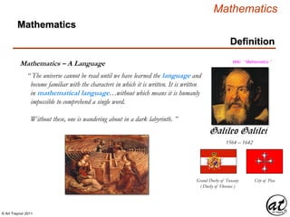
Galileo Galilei
Grand Duchy of Tuscany
( Duchy of Florence )
City of Pisa
Mathematics – A Language
“ The universe cannot be read until we have learned the language and
become familiar with the characters in which it is written. It is written
in mathematical language…without which means it is humanly
impossible to comprehend a single word.
Without these, one is wandering about in a dark labyrinth. ”

© Art Traynor 2011
Mathematics
Definition
Algebra – A Mathematical Grammar
Mathematics
A formalized system ( a language ) for the transmission of
information encoded by number
Algebra
A system of construction by which
mathematical expressions are well-formed
Expression
Symbol Operation Relation
Designate expression
elements or Operands
Transformations capable of
rendering an expression
into a relation
A mathematical structure
between operands
represented by a well-formed
expression
A well-formed symbolic representation of operands, of discrete arity, upon which one
or more operations can structure a Relation
1. Identifies the explanans
by non-tautological
correspondences
Definition
2. Isolates the explanans
as a proper subset from
its constituent
correspondences
3. Terminology
a. Maximal parsimony
b. Maximal syntactic
generality
4. Examples
a. Trivial
b. Superficial
Mathematics

© Art Traynor 2011
Mathematics
Disciplines
Algebra
One of the disciplines within the field of Mathematics
Mathematics
Others are Arithmetic, Geometry,
Number Theory, & Analysis

The study of expressions of symbols ( sets ) and the
well-formed rules by which they might be consistently
manipulated.

Algebra
Elementary Algebra
Abstract Algebra
A class of Structure defined by the object Set and
its Operations

Linear Algebra
Mathematics

© Art Traynor 2011
Mathematics
Definitions
Expression
into a relation
A mathematical structure
between operands
represented by a well-formed
expression
A well-formed symbolic representation of operands, of discrete arity, upon which one
or more operations may structure a Relation
Expression – A Mathematical Sentence
Proposition
A declarative expression
asserting a fact, the truth
value of which can be
ascertained
Formula
A concise symbolic
expression positing a relationVariablesConstants
An alphabetic character
representing a number the
value of which is arbitrary,
unspecified, or unknown
Operands ( Terms )
A transformation
invariant scalar quantity
Mathematics

© Art Traynor 2011
Mathematics
Definitions
Expression
into a relation
A mathematical structure between operands represented
by a well-formed expression
Proposition
asserting a fact, the truth
value of which can be
ascertained
Formula
A concise symbolic
expression positing a relation
VariablesConstants
An alphabetic character
representing a number the
value of which is arbitrary,
unspecified, or unknown
Operands ( Terms )
A transformation
invariant scalar quantity
Equation
A formula stating an
equivalency class relation
Inequality
A formula stating a relation
among operand cardinalities
Function
A Relation between a Set of inputs and a
Set of permissible outputs whereby each
input is assigned to exactly one output
Univariate: an equation containing
only one variable
Multivariate: an equation containing
more than one variable
(e.g. Polynomial)
Mathematics

© Art Traynor 2011
Mathematics
Definitions
Expression
Proposition Formula
VariablesConstants
Operands ( Terms )
Equation
A formula stating an
equivalency class relation
Linear Equation
An equation in which each term is either
a constant or the product of a constant
and (a) variable[s] of the first order
Mathematics

© Art Traynor 2011
Mathematics
Expression
Mathematical Expression
A Mathematical Expression is a precursive finite composition
to a Mathematical Statement or Proposition
( e.g. Equation) consisting of:

a finite combination of Symbols
possessing discrete Arity
Expression
A well-formed symbolic
representation of operands, of
discrete arity, upon which one
or more operations can
structure a Relation
that is Well-Formed
Mathematics

© Art Traynor 2011
Mathematics
Arity
Arity
Expression
The enumeration of discrete symbolic elements ( Operands )
comprising a Mathematical Expression is defined as
its Arity

The Arity of an Expression is represented by
a non-negative integer index variable ( ℤ + or ℕ ),
conventionally “ n ”

A Constant ( Airty n = 0 , index ℕ )or Nullary
represents a term that accepts no Argument

A Unary or Monomial has Airty n = 1
VariablesConstants
Operands
Expression
A relation can not be defined for
Expressions of arity less than
two: n < 2
A Binary or Binomial has Airty n = 2
All expressions possessing Airty n > 1 are Polynomial
also n-ary, Multary, Multiary, or Polyadic


© Art Traynor 2011
Mathematics
Arity
Arity
Expression
VariablesConstants
Operands
Expression
A relation can not be defined for
Expressions of arity less than
two: n < 2
Nullary
Unary
n = 0
n = 1 Monomial
Binary n = 2 Binomial
Ternary n = 3 Trinomial
1-ary
2-ary
3-ary
Quaternary n = 4 Quadranomial4-ary
Quinary n = 5 5-ary
Senary n = 6 6-ary
Septenary n = 7 7-ary
Octary n = 8 8-ary
Nonary n = 9 9-ary
n-ary

© Art Traynor 2011
Mathematics
Equation
Equation
Expression
An Equation is a statement or Proposition
( aka Formula ) purporting to express
an equivalency relation between two Expressions :

Expression
Proposition
asserting a fact whose truth
value can be ascertained
Equation
A symbolic formula, in
the form of a proposition,
expressing an equality
relationship
Formula
A concise symbolic
expression positing a
relationship between
quantities
VariablesConstants
Operands
Symbols
Operations
The Equation is composed of Operand terms and
one or more discrete Transformations ( Operations )
which can render the statement true

© Art Traynor 2011
Mathematics
Equation

Expression
Proposition
Equation
relationship
Formula
A concise symbolic
quantities
Polynomial
Polynomial
An Equation with LOC set consisting of
the arithmetic Transformations
( excluding negative exponentiation )
LOC ( Pn ) = { + , – , x bn ∀ n ≥ 0 , ÷ }
A Term of a Polynomial Equation is a compound
construction composed of a coefficient and variable
in at least one unknown
Polynomial
Equation

© Art Traynor 2011
Mathematics
Equation

Expression
Proposition
Equation
relationship
Formula
A concise symbolic
quantities
Polynomial
Polynomial
Σ an xi
n
i = 0
P( x ) = an xn + an – 1 xn – 1 +…+ ak+1 xk+1 + ak xk +…+ a1 x1 + a0 x0
Variable
Coefficient
Polynomial Term
Polynomial
Equation

© Art Traynor 2011
Mathematics
Linear Equation
Linear Equation
Equation
An Equation consisting of:
Operands that are either
Any Variables are restricted to the First Order n = 1
Linear Equation
An equation in which each term
is either a constant or the
product of a constant and (a)
variable[s] of the first order
Expression
Proposition
Equation
Formula
n Constant(s) or
n A product of Constant(s) and
one or more Variable(s)
The Linear character of the Equation derives from the
geometry of its graph which is a line in the R2 plane

As a Relation the Arity of a Linear Equation must be
at least two, or n ≥ 2 , or a Binomial or greater Polynomial


© Art Traynor 2011
Mathematics
Linear Equation
Equation
Standard Form ( Polynomial )
 Ax + By = C
 Ax1 + By1 = C
For the equation to describe a line ( no curvature )
the variable indices must equal one

 ai xi + ai+1 xi+1 …+ an – 1 xn –1 + an xn = b
 ai xi
1 + ai+1 x 1 …+ an – 1 x 1 + a1 x 1 = bi+1 n – 1 n n
ℝ
2
: a1 x + a2 y = b
ℝ
3
: a1 x + a2 y + a3 z = b
Blitzer, Section 3.2, (Pg. 226)
Section 1.1, (Pg. 2)
Test for Linearity
 A Linear Equation can be expressed in Standard Form
As a species of Polynomial , a Linear Equation
can be expressed in Standard Form
 Every Variable term must be of precise order n = 1

© Art Traynor 2011
Mathematics
Operand
Arity
Operand
the object of a mathematical operation,
a quantity on which an operation is performed
 Arithmetic: a +b = c
Within an expression or set
 “a” and “b” are Operands
 The number of Operands of an Operator is known as its Arity
n Nullary = no Operands
n Unary = one Operand
n Binary = two Operands
n Ternary = three Operands…etc.
In other words…
Operands
“Belong To”
their Operators

© Art Traynor 2011
Mathematics
Linear Equation
Equation
Standard Form
 Ax + By = C
 Ax1 + By1 = C
For the equation to describe a line ( no curvature )
the variable indices must equal one

 ai xi + ai+1 xi+1 …+ an – 1 xn –1 + an xn = b
 ai xi
1 + ai+1 x 1 …+ an – 1 x 1 + a1 x 1 = bi+1 n – 1 n n
ℝ
2
: a1 x + a2 y = b
ℝ
3
: a1 x + a2 y + a3 z = b

© Art Traynor 2011
Mathematics
Definition
Differential Equation
Differential Equations
A Differential Equation is one containing a Derivative or Differential of one or more
Dependent variables with respect to one or more independent variables
A Differential Equation is a mathematical equation for an unknown function of one or
several variables that relates the values of the function itself and its derivatives of various orders
Differential Equations arise from the mathematical description/specification of
phenomena, modeled by functions, stated in terms implying deterministic relations between one or
more variables, wherein the essence of the relationship known or postulated, entails a rate of
change (expressed as one or more derivatives).
Differential Equations arise from…
They are the mathematical form best suited to model the underlying relationship.
Why a differential equation?*

© Art Traynor 2011
Mathematics
Definition
A Differential Equation is one
with respect to
of one or more dependent variables
one or more independent variables
Z&C Definition 1.1containing a Derivative or Differential
A Differential Equation is a mathematical equation
that relates
of one or several variables
the values of the function itself
for an unknown function
And its derivatives of various orders
 Has to have a derivative
 Pre-supposes implicit
relationships
Qualifications

© Art Traynor 2011
Mathematics
Solutions
Differential Equation Solution
Any function f,
defined on some interval I,
reduces the equation to an Identity
which when substituted into a Differential Equation
 f(x) = y =
x 4
16
 dy/dx = xy1/2
The “ function” which provides the “ solution ” to the DE
The DE to be solved
Note:
DE is Ordinary – only one dep variable
The ODE is Linear – the dependent
variable and any of its derivatives are of a
degree no greater than one
*
*
Dx (cxn ) = (cn)x n-1f(x) = y =
1
16
x4 4
16
x3 1
4
x3
Find the derivative of
the putative solution
f´(x) = dy/dx =
1
4
x3 or
x 3
4
dy/dx - xy½ = xy½ - xy½ dy/dx - xy½ = 0 Set the DE equal to zero

© Art Traynor 2011
Mathematics
Differential Equation Solution
 f(x) = y =
x 4
16
 dy/dx = xy1/2
The “ function” which provides the (explicit) “ solution ” to the DE
The DE to be solved
Dx (cxn ) = (cn)x n-1f(x) = y =
1
16
x4 4
16
x3 1
4
x3
Find the derivative of
f´(x) = dy/dx =
1
4
x3 or
x 3
4
dy/dx - xy½ = xy½ - xy½ dy/dx - xy½ = 0 Set the DE equal to zero
Plug the derivative of the
putative solution into the DE
dy/dx - x · y½ = 0
x 3
4
- xy½ = 0
Plug the expression for f(x) = y into the
DE (to obtain an expression
exclusively in terms of the independent
variable)
x 3
4
- x
½
x 4
4 = 0
x 3
4
- x
√¯
16
√¯
x 4
x 3
4
- x= 0 x 2
4
= 0
x 3
4
- x 3
4
= 0 Q.E.D.
Solutions

© Art Traynor 2011
Mathematics
Differential Equation “ Particular ” Solution
 f(x) = y = cex
 dy/dx = y´ = y
The “ function ” which provides the
(explicit) solution ” to the DE
The DE to be solved
Dx (cxn ) = (cn)x n-1f(x) = y = cex Find the derivative of
f´(x) = y´ = y
Solutions
c Dx (ex) =
dy
dx
= y´ = cex
f(x) = cex = cex
Plug the derivative of
into the D.E. to verify
Identity
For c = 0
-2
5
y =
DE Scorecard
Is this an ODE or PDE?*0
-2ex
5ex
dy/dx = y´ = y
DE has only one independent variable = ODE
DE Scorecard
ODE or PDE?
Order?
*
*
Linear or Non-Linear?*
ODE

© Art Traynor 2011
Mathematics
 f(x) = y = cex
 dy/dx = y´ = y
f´(x) = y´ = y
Solutions
c Dx (ex) =
dy
dx
= y´ = cex
f(x) = cex = cex
Identity
For c = 0
-2
5
y = 0
-2ex
5ex
DE Scorecard
dy/dx = y´ = y
Can DE be written in the following form:
The DE to be solved
DE Scorecard
ODE or PDE?
Order?
*
*
ODE
What Order is this DE?*
dny
dxnan(x)
1
+…+
d0y
dx0a0(x) = g(x)
1

© Art Traynor 2011
Mathematics
 f(x) = y = cex
 dy/dx = y´ = y
f´(x) = y´ = y
Solutions
c Dx (ex) =
dy
dx
= y´ = cex
f(x) = cex = cex
Identity
For c = 0
-2
5
y = 0
-2ex
5ex
DE Scorecard
dy/dx = y´ = y = a0(x0)
The DE to be solved
DE Scorecard
ODE or PDE?
Order?
*
*
ODE
What Order is this DE?*
d1y
dx1 = f(x)
1
Determines DE Order (n=Order)
Order = 1
The Order of the DE also
determines the number of
parameters in the family of
solutions (e.g. if n=1, c=1)

© Art Traynor 2011
Mathematics
 f(x) = y = cex
 dy/dx = y´ = y
f´(x) = y´ = y
Solutions
c Dx (ex) =
dy
dx
= y´ = cex
f(x) = cex = cex
Identity
For c = 0
-2
5
y = 0
-2ex
5ex
DE Scorecard
The DE to be solved
DE Scorecard
ODE or PDE?
Order?
*
*
ODE
Is this DE Linear or Non-Linear?*
1
Determines Linearity 1
dy/dx = y´ = y = a0(x0)
d0y
dx0 = f(x)
1
All derivative terms are indexed by 1 = Linear

© Art Traynor 2011
Mathematics
 f(x) = y = cex
 dy/dx = y´ = y
f´(x) = y´ = y
Solutions
c Dx (ex) =
dy
dx
= y´ = cex
f(x) = cex = cex
Identity
For c = 0
-2
5
y = 0
-2ex
5ex
(explicit) solution to the DE
The DE to be solved
DE Scorecard
ODE or PDE?
Order?
*
*
ODE
1
Linear
Test for an(xn)
d ny
dxn = g(x) form
1
y´ = y y´ - y = 0
a0(x0) can be introduced as the parametric
and independent variable terms as identities
dy/dx = y´ = a0(x0) y´
Highest order derivative term a0(x0)
d 1y
dx1
1
Particular Solutions
Arbitrary Parameter
Often specified to fulfill
“Initial/Boundary” conditions
A “General/Complete Solution”
for the nth-order, n-parameter
FAMILY of solutions to the DE
(n=c=1)

© Art Traynor 2011
Mathematics
Classifications
Differential Equation Classifications
 Type
 Order
 Linearity

© Art Traynor 2011
Mathematics
Classifications
 Type
 Order
 Linearity
 Ordinary Differential Equation (ODE)
 Partial Differential Equation (PDE)
The highest order derivative (of the dependent variable) of a differential
equation determines the order of the equation
A differential equation containing terms of only dependent variable
A differential equation containing terms of two or more dependent variables
 Linear
 Non-Linear
A differential equation violating any of the two “linear” definition constraints
n The dependent variable y and all its derivatives within the differential equation are only of the
first degree (i.e. the power of each term involving y is one)
n Each coefficient depends only on the independent variable x
 Codes relations beyond the
principal (rate of change or
change of rate)??

© Art Traynor 2011
Mathematics
Classifications
 Type
 Ordinary Differential Equation (ODE)
 Partial Differential Equation (PDE)
A differential equation containing terms of only dependent variable
A differential equation containing terms of two or more dependent variables
“Type” addresses the question “what are the determinants of the DE”
e.g. Are they of a singular or multiple independent influence?

© Art Traynor 2011
Mathematics
Classifications
 Order
“Order” addresses the question “what is the nature of the DE relation”
e.g. Is it a rate of change? Is it a change in a rate?
 The Order of the DE also determines the number of parameters in the family of
solutions, (e.g. where yn means dny/dxn we expect an n-parameter family of solutions).
 A solution of a DE free of arbitrary parameters (e.g. of the type f(x) = cex ) is said
to be a Particular Solution of the DE, often specified to fulfill initial/boundary conditions
Arbitrary Parameter
 Where a particular solution (to an initial/boundary condition) fails to yield a unique
solution (i.e. specializing the parameters) that solution set (as small as a single point or
as large as the full real line) is said to constitute a singular solution (or one at which
there is said to be a failure of uniqueness).

© Art Traynor 2011
Mathematics
Classifications
 Order
 The Order of the DE also determines the number of parameters in the family of
solutions, (e.g. where yn means dny/dxn we expect an n-parameter family of solutions).
 A solution of a DE free of arbitrary parameters (e.g. of the type f(x) = cex ) is said
to be a Particular Solution of the DE, often specified to fulfill initial/boundary conditions
Arbitrary Parameter
 Where a particular solution (to an initial/boundary condition) fails to yield a unique
solution (i.e. by means of specializing the parameters) that solution set (as small as a
single point or as large as the full real line) is said to constitute a singular solution
(or one at which there is said to be a failure of uniqueness). This singular solution
represents the envelope of the family of solutions to the DE.
 A general or complete solution is one in which the constants are expressed in an
undetermined form (contrasted with a particular solution where the constants are defined).

© Art Traynor 2011
Mathematics
Classifications
 Linearity
 Linear
 Non-Linear
A differential equation violating any of the two “linear” definition constraints
n The dependent variable y and all its derivatives within the differential equation are only of the
first degree (i.e. not exceeding the power of one)
n Each coefficient depends only on the independent variable x
dny
dxnan(x) + an-1(x)
dn-1y
dxn-1 +…+
dy
dx
a1(x) + a0(x) y = g(x)
 Test
A DE is Linear if it can be written in the following form:
dny
dxnan(x)
1
+ an-1(x)
dn-1y
dxn-1 +…+ a1(x)
d1y
dx1
d0y
dx0+ a0(x) = g(x)
111

© Art Traynor 2011
Mathematics
Linear Equation
Section 2.5, (Pg. 62)Integrating Factor ( IF )
An Integrating Factor is an extraneous function [ M(x) or μ(x) ] introduced into a
differential equation to facilitate the solution of the system by means of integration.
The IF is specified so that the ratio of the extraneous function derivative and the
variable [ P(x) ].
M´(x)
M(x)
extraneous function are equal to the coefficient function of the dependent
The integration of this equality thus results in the IF that allows for further
integration of the system (by IBP, Substitution, etc.) to yield a solution.

© Art Traynor 2011
Mathematics
Linear Equation
dny
dxnan(x) + an-1(x)
dn-1y
dxn-1 +…+
dy
dx
a1(x) + a0(x) y = g(x)
Beginning with the generalized form of a Linear Differential Equation ( LDE )
dny
dxnan(x)
1
+ an-1(x)
dn-1y
dxn-1 +…+ a1(x)
d1y
dx1
d0y
dx0+ a0(x) = g(x)
111
For n = 1 the generalized LDE form reduces to a
Linear First Order Differential Equation ( LFODE )
1. Each coefficient may
only be functions of the
independent variable
DE Linearity Criteria
2. The degree of the
dependent variable and
all its derivatives is
precisely equal to one
For a Linear Equation, an Integrating Factor can be derived by the following process:


dy
dx
a1(x) + a0(x) y = g(x) Restatement of general expression for n = 1

© Art Traynor 2011
Mathematics
Linear Equation
For n = 1 the generalized LDE form reduces to a
Linear First Order Differential Equation ( LFODE )

dy
dx
a1(x) + a0(x) y = g(x)
Restatement of
general expression
for n = 1
a1(x)
1
a1(x)
1
dy
dx
+ y = g(x)
a1(x)
1
dy
dx
+ y = g(x) a1(x)
1
a1(x)
1 a1(x)
1
dy
dx
+ y = g(x) a1(x)
1
①
a1(x)
a0(x)
a0(x)
1
a1(x)
1 a0(x)
1
dy
dx
+ (x) y = g(x) a1(x)
1
a1(x)
a0(x)
Somehow or other
the (x) is factored out
of it’s reconfigured
coefficient ratio??

© Art Traynor 2011
Mathematics
Linear Equation
Substitution of the coefficient function of the dependent variable a0(x)
with a more conventional form [ P(x) ] yields

The text (as usual)
skips crucial steps,
so it’s not clear how
these terms
disappear, but
vanish, they do…
dy
dx
+ (x) y = g(x) 1
1
1
1
dy
dx
+ (x) y = g(x)
The simplified
expression is thus
restated into a more
“conventional” form
with Y as P(x) and
g(x) as f(x)
dy
dx
dy
dx
+ (x) y = g(x) a1(x)
1
a1(x)
a0(x)
+ P(x) y = f (x)

© Art Traynor 2011
Mathematics
Linear Equation
Substitution of the coefficient function of the dependent variable a0(x)
with a more conventional form [ P(x) ] yields

dy
dx
+ P(x) y = f (x)
Once rendered into this form, we can trace the additional steps necessary to
derive an appropriate expression for the extraneous function [ M(x) or
μ(x) ] by which the integration of the function can proceed.

The derivation begins by migrating the f (x) term from the RHS to the
LHS to restate the “conventional” form as a Homogenous Linear
Differential Equation ( HLDE )
①
dy
dx
+ P(x) y – f (x) = 0
Note that the IF here is
applicable to a FOLDE
featuring “Constant”
coefficients, a similar
method “Variation of
Parameters” ( VOP see
page 195 ) is available
for “Variable” coefficients

© Art Traynor 2011
Mathematics
Linear Equation

The migrated HLDE can then be differentiated with respect to the
independent variable “ x ”
dy
dx
Dx + P(x) y – f (x) = 0
dy
dx
+ P(x) y – f (x) = 01
dx
②
The differential ratio form
algebraic manipulation of
the LFODE into a form
where the extraneous
function can be introduced
dy
dx
works very well
here to facilitate
dy
dx
+ P(x) y – f (x) = 01
dx
1
dx
1
dx
dy + P(x) y – f (x) dx = 0

© Art Traynor 2011
Mathematics
Linear Equation

Stated in this modified differential form, the extraneous function can
now be introduced [ M (x) or μ (x) ]
dy + P(x) y – f (x) dx = 0
③
μ(x) dy + μ(x) P(x) y – f (x) dx = μ(x) 0
The introduction of the
extraneous function is
permitted as a
consequence of the
properties of an Exact
Differential (see pg 55)

© Art Traynor 2011
Mathematics
Linear Equation
The extraneous function is now verified as an exact differential by
equating partial derivatives of the terms of the LHS of the equation
μ(x) dy + μ(x) · P(x) y – f (x) dx = μ(x) 0
④
Left Hand Side ( LHS )
μ(x) dy = μ(x) · P(x) y – f (x) dx∂
∂x
1. Why only consider the
LHS? Why not move
one term to RHS and
evaluate as a equality?
Abiguities
2. What becomes of the
standard differentials –
dx & dy?
∂
∂y
μ(x) dy = μ(x) · P(x) y – y dx∂
∂x
∂
∂y
Replacing “ f (x) ” with
“ y ” as f (x) = y
dy = μ(x) P(x) y – y dx
dμ
dx
∂
∂y Dx ( x n ) = n x n – 1
dy = μ(x) P(x) 1 – 1 dx
dμ
dx
Constants with respect
to the “partial” can be
commuted outside the
argument of the
differential operator

© Art Traynor 2011
Mathematics
Linear Equation
By continued algebraic manipulation, we see that the equated partial
derivative terms reduce to an equivalency between the dependent
variable term [ P(x) ] and the ratio of the extraneous function
derivative to its functional value.
dy = μ(x) P(x) dx
dμ
dx
μ(x) · P(x) =dx
dμ
dx
P(x) =dx
dμ
dx
μ(x)
1μ(x)
1
μ(x)
1
P(x) = μ´(x)
μ(x)
1μ(x)
1
μ(x)
1
P(x) = μ(x)
μ ´(x)
4a
Transitioning from
dy
dx
(differential ratio) notation to
f´(x) form (prime function)
form to more fully elucidate
the ratio equivalency of the
extraneous function
Z&C rates this as a
“Separable Equation”

© Art Traynor 2011
Mathematics
Linear Equation
In this step we will further refine the expression equating the ratio of
the extraneous function derivative to its functional value ( LHS )
and the LFODE dependent variable coefficient function ( RHS )
P(x) = μ(x)
μ ´(x)
4b
Left Hand Side ( LHS ) Right Hand Side ( RHS )
μ(x)
1
P(x) =
dμ
dx
The f´(x) form (prime
function) of the derivative
μ´(x) is restated in dy
dx(differential ratio)
form so as to allow us to
manipulate it algebraically
μ(x)
1
μ(x) P(x) =
dμ
dx 1
μ(x)
μ(x) · P(x) =
dμ
dx
dy = μ(x) P(x) dx
dμ
dx

© Art Traynor 2011
Mathematics
Linear Equation
The ratio expression of the extraneous function, equated to the
LFODE dependent variable coefficient function, must be further
manipulated to permit integration of the equation (which supplies
the IF – in its proper form - to be substituted back into the LFODE
and multiplied by its remaining terms)
dy = μ(x) · P(x) dx
dμ
dx
dy = μ(x) · P(x) dx
dμ
dx
dx
1
dx
1
dy dμ = μ(x) · P(x) · dx dx
dy = · P(x) · dx dx
dμ
1μ(x)
1
dy = P(x) · dx dx
dμ
μ(x)
1
μ(x)
μ(x)
1
1
μ(x)
dy = P(x) · dx dx
dμ
μ(x)
4c
Z&C rates this as a
“Separable Equation”
Here we will stick with the
differential ratio notation
dy
dx
allowing us to separate
the differential operator
algebraically to a form where
integration can be employed
to obtain an expression for
the extraneous function that
can then be introduced into
the differential equation
substituting for its dependent
variable coefficient.

© Art Traynor 2011
Mathematics
dy dμ = P(x) · dx dx
Linear Equation
The equation is now in a state where, with some minor additional
manipulation, it can be integrated to yield the IF to be substituted in
place of the LFODE dependent variable coefficient function and
multiplied by each of the other terms of the LFODE.
dy = P(x) · dx dx
dμ
μ(x)
μ(x)
1 Separate the LHS vinculum
expression in preparation for
integration of the equatioin
dy dμ = P(x) · dx dxμ(x)
1
∫ ∫
dy ln | μ | = P(x) · dx dx
∫
5a

© Art Traynor 2011
Mathematics
Linear Equation
The equation is now in a state where, with some minor additional
manipulation, it can be integrated to yield the IF to be substituted in
place of the LFODE dependent variable coefficient function and
multiplied by each of the other terms of the LFODE.
5b
dy ln | μ | = P(x) · dx dx
∫
dy ln | μ | = P(x) · dx dx∫e e
μ(x) = e ∫ P(x)dx
dx

© Art Traynor 2011
Mathematics
Linear Equation
dy
dx
+ P(x) y = f (x)
The IF is introduced into the LFODE first by substitution for the
dependent variable coefficient function and then as a multiplier for
each of the remaining two terms of the LFODE.
⑥
dy
dx e ∫ P(x)dx
+ e ∫ P(x)dx
y = f (x) e ∫ P(x)dx

© Art Traynor 2011
Mathematics
Integration
Calculus
Integration by Parts ( IBP )
Example: Solve the Initial Value Problem ( IVP ) Section 2.5, (Pg. 67),
Example 6
The equation must first be classified according to the following criteria:①
a
=
dy
dx
1
x + y2
y ( – 2 ) = 0
Separable?
b Homogenous?
c Exact?
d Linear?
This equation fails each test, however, its reciprocal admits a linear
relation in “ x ” ( i.e. not “y”, as is conventional, requiring a “change of
variable” with respect to the IF )
=
dx
dy 1
x + y2
→ = x + y2
dx
dy
→ – x = y2
dx
dy

© Art Traynor 2011
Mathematics
Integration
Calculus
Example 6
The equation must next be manipulated into a LFODE form where the
dependent variable coefficient function can be identified for
substitution with the appropriate IF
– x = y2dx
dy → – y0 x = y2dx
dy
②
+ P( y ) x = f ( y )
dx
dy
After rudimentary manipulation,
it is readily apparent that the
value of P ( y ) is a constant
value of – 1
μ( y ) = e ∫ P( y ) dy
dx
μ( y ) = e ∫ [ –1 ] dy
dx
μ( y ) = e
– ∫ dy
dx e
– y
dx→
+ e
– y
dx = y 2
dx
dy
P( y ) = – 1

© Art Traynor 2011
Mathematics
Integration
Calculus
Example 6
The IF once identified must then be applied as a multiplier to the
remaining terms of the LFODE
– x = y2dx
dy → – y0 x = y2dx
dy
+ P( y ) x = f ( y )
dx
dy
After rudimentary manipulation,
it is readily apparent that the
value of P ( y ) is a constant
value of – 1
+ e
– y
dx = y 2
dx
dy
e
– y
+ e
– y
d x = y 2 e
– ydx
dy
This equation, substituted for the
IF, represents the RESULT of a
“Product Rule” differentiation
…identifying those terms in
sequence, the PR differentiation
can thus be reversed by
identifying the terms of the PR
differentiation
③

© Art Traynor 2011
Mathematics
Integration
Calculus
Example 6
The equation must next be manipulated into a LFODE form where the
dependent variable coefficient function can be identified for
substitution with the appropriate IF
e
– y
+ e
– y
d x = y 2 e
– ydx
dy
This equation, substituted for the
IF, represents the RESULT of a
“Product Rule” differentiation
…identifying those terms in
sequence, the PR differentiation
can thus be reversed by
identifying the terms of the PR
differentiation
④

© Art Traynor 2011
Mathematics
Constant Coefficient DE’s
Homogenous Linear Differential Equation
Section 1.1 (Pg. 3)
Constant Coefficient
Diffferential Equations
( CCDE )A Homogenous Linear Differential Equation ( HLDE ) formatted such that its
Terms ( proceeding from L → R ) decrease in order by an increment of negative
unity is said to be in Unity-Decremented Order Term Form ( UDOTF ) : Section 4.3 (Pg. 159)
Section 6.1 (Pg. 258)
dny
dxnan(x·n + an-1(x·)
dn-1y
dxn-1 +…+
dy
dx
a1(x· + a0(x· y = 0
dny
dxn
1
+ an-1(x)·n dn-1y
dxn-1 +…+ a1(x· 1 d1y
dx1
d0y
dx0+ a0(x)· 0 = 0
111
Determines
Linearity 1
an(x·
As a Linear Equation, it is apparent on reflection that any plausible
solution must feature an expression, the terms of which will not be
altered in form by successive differentiation or integration.
The exponential function ( and its composites ) can thus be readily seen
as satisfying this necessity.

All Solutions
of UDOTF equations
feature solutions that are
exponential functions
or compositions of
exponential functions

© Art Traynor 2011
Mathematics
Section 1.1 (Pg. 3)
dny
dn-1y
dxn-1 +…+
dy
dx
a1(x· + a0(x· y = 0
dny
dxn
1
+ an-1(x)·n dn-1y
dxn-1 +…+ a1(x· 1 d1y
dx1
d0y
dx0+ a0(x)· 0 = 0
111
Determines
Linearity 1
an(x·
Special Cases
 First Order Linear Homogenous Differential Equation ( FOLHDE )
d 2y
dx2an(x)2 + a1 (·
dy
dxn-1 +
dy
dx
a1(x) 1 + a00( · y = 0
d2y
dx2an(x)2 + a1 (·
dy
dxn-1 + a0 y = 0
n
Always features the solution: d y = c1 e
– a0
x Section 4.3 (Pg. 159)
Leading coefficient a1 = 1

© Art Traynor 2011
Mathematics
Section 1.1 (Pg. 3)
Special Cases
an(x)2 dy
dxn-1 + a0 y = 0 y = c1 e
– a0
x
a1 ·
y0 = Dx [ c1 e – a0
x
]
The exponential solution for the dependent variable of the UDOTF
FOLHDE can then be rendered into a chart, where through
successive differentiation, differential terms directly corresponding to
each of the terms of the FOLHDE can be arrayed

y0 = c1 e–a0
x
dy
dxn
Dx [ eu ] = eu Dx [ u ]
Chain Rule for Exponential Differentiation
Dx [ xn ] = n xn – 1
Power Rule for Derivatives

© Art Traynor 2011
Mathematics
Section 1.1 (Pg. 3)
( CCDE )
Special Cases
an(x)2 dy
dxn-1 + a0 y = 0a1 ·
y0 = Dx [ c1 e – a0
x
]
Chart of corresponding exponential differential terms
y0 = c1 e–a0
x
dy
dxn
y0 = c1 Dx [ e – a0
x
]
dy
dxn
e CR Substitution
u du
Dx [ eu ] = eu Dx [ u ]
– a0 x1 – 1a0 x0
Dx [ xn ] = n xn – 1
– a0 x – 1a0 x0y0 = c1 Dx [ e u
]
dy
dxn
y0 = c1 e u
Dx [ ue u
]
dy
dxn
y = c1 e
– a0
x

© Art Traynor 2011
Mathematics
Section 1.1 (Pg. 3)
( CCDE )
Special Cases
an(x)2 dy
dxn-1 + a0 y = 0 y = c1 e
– ax
a1 ·
y0 = c1 e–a0
x Dx [ eu ] = eu Dx [ u ]
Dx [ xn ] = n xn – 1
y0 = c1 e u
· Dx [ ue u
]
dy
dxn
y0 = c1 e – a0
x
Dx [ – a0 x ]
dy
dxn
y0 = – a0 c1 e – a0
x
Dx [ – ax ]
dy
dxn
y0 = – a0 c1 e – a x
· ( 1 )
dy
dxn
y0 = – a0 c1 e – a x
· ( 1 )
dy
dxn
e CR Substitution
u du
– a0 x1 – 1a0 x0
– a0 x – 1a0 x0

© Art Traynor 2011
Mathematics
Section 1.1 (Pg. 3)
( CCDE )
Special Cases
an(x)2
Dx [ eu ] = eu Dx [ u ]
Dx [ xn ] = n xn – 1
y0 = c1 e u
· Dx [ ue u
]
dy
dxn
y0 = c1 e – a0
x
Dx [ – ax ]
dy
dxn
y0 = – ac1 e – a0
x
Dx [ – ax ]
dy
dxn
y0 = – ac1 e – a0
x
· ( 1 )
dy
dxn
y0 = – ac1 e – a0
xdy
dxn
e CR Substitution
u du
– a0 x1 – 1a0 x0
– a0 x – 1a0 x0
y = c1 e–a0
x
dy
dxn-1 + a0 y = 0a1 · y = c1 e
– a0
x

© Art Traynor 2011
Mathematics
Section 1.1 (Pg. 3)
( CCDE )
Special Cases
an(x)2

y0 = c1 e–a0
x
y0 = – a0 c1 e – a0
xdy
dxn
an(x)2
dy
dxn-1 + a0 y = 0a1 ·
We can verify these
corresponding
exponential differential
terms satisfy our
FOLHDE by
substituting them into
the FOLHDE itselfa1 [ – a0 c1 e – a0 x
] + a0 [ c1e –a0
x
] = 0
For a1 = 1
1 [ – a0 c1 e – a0 x
] + a0 [ c1e
–a0
x
] = 0
dy
dxn-1 + a0 y = 0a1 · y = c1 e
– a0
x
Chart of corresponding exponential differential terms
1 [ – a0 c1 e – a0 x
] + a0 · c1e
–a0
x
] = 0
0] = 0 QED

© Art Traynor 2011
Mathematics
Section 1.1 (Pg. 3)
Special Cases
 Second Order Linear Homogenous Differential Equation ( SOLHDE )
d 2y
dx2an( ·)2 + b ( · 1 dy
dxn-1 +
dy
dx
a1(x) 1 + c0(x)· y = 0
d2y
dx2an( ·)2 + b ( ·1 dy
dxn-1 + c y = 0
dny
dn-1y
dxn-1 +…+
dy
dx
a1(x· + a0(x· y = 0
dny
dxn
1
+ an-1(x)·n dn-1y
dxn-1 +…+ a1(x· 1 d1y
dx1
d0y
dx0+ a0(x)· 0 = 0
111
Determines
Linearity 1
an(x·

© Art Traynor 2011
Mathematics
Section 1.1 (Pg. 3)
( CCDE )
Special Cases

y0 = c1 e–a0
x
y0 = – a0 c1 e – a0
xdy
dxn
an(x)2
Let – a0 = m
y = c1 e
– a0
x
Chart of corresponding exponential differential terms
d2y
dx2an( ·)2 + b ( ·1 dy
dxn-1 + c y = 0
y = c1 e
mxd2y
dx2an( ·)2 + b ( ·1 dy
dxn-1 + c y = 0
y0 = Dx [ c1 e – a0
x
]
d2y
dx2
n
Let – a0 = m
→
→
→
c1 · emx
c1 me mx
yDx [ c1 · em x
]

© Art Traynor 2011
Mathematics
Section 1.1 (Pg. 3)
( CCDE )
Special Cases
e CR Substitution
u du
Dx [ eu ] = eu Dx [ u ]
mx1 m(1)
Dx [ xn ] = n xn – 1
m0
0
y = c1 e
mxd2y
dx2an( ·)2 + b ( ·1 dy
dxn-1 + c y = 0
y0 =
y0 =
dy
dxn
y0 =
d2y
dx2
n
c1 · emx
c1 me mx
yDx [ c1mem x
] → yDx [ c1 m em x
]
c1 m y Dx [ em x
]
c1 m yv Dx [ eu x
]
c1 m eu
Dx [ u
u x
]

© Art Traynor 2011
Mathematics
Section 1.1 (Pg. 3)
( CCDE )
Special Cases
e CR Substitution
u du
Dx [ eu ] = eu Dx [ u ]
mx1 m(1)
Dx [ xn ] = n xn – 1
m0
0
y = c1 e
mxd2y
dx2an( ·)2 + b ( ·1 dy
dxn-1 + c y = 0
y0 =
y0 =
dy
dxn
y0 =
d2y
dx2
n
c1 · emx
c1 me mx
yDx [ c1mem x
] →
c1 m em x
Dx [ m x ]
c1 m eu
Dx [ u
u
]
c1 m2 em x
Dx [ m x ]
c1 m2 em x
· ( m 1 )

© Art Traynor 2011
Mathematics
Homogenous Linear Differential Equation Section 1.1 (Pg. 3)
Special Cases
y = c1 e
mxd2y
dx2an( ·)2 + b ( ·1 dy
dxn-1 + c y = 0
y0 =
y0 =
dy
dxn
y0 =
d2y
dx2
n
c1 · emx
c1 m·e mx
c1 m2 em x
dy
dxn-1a · + b · + c · y = 0
Substituting these
exponential differential
terms back into our
SOLHDE renders the
SOLHDE into a form
from which a solution
can in turn be foundd2y
dx2
n
a · c1 m2 em x
+ b · c1 mem x
+ c · c1 · emx
= 0
Factoring
common
terms
c1em x
[ a · m2 + b · m + c ] = 0
c1em x
[ am2 + bm + c ] = 0 As the exponential function can never
equate to zero, the roots of this
Auxiliary or Characteristic Equation
polynomial supply the solutions to the
complementary function yc

© Art Traynor 2011
Mathematics
Distinct Real Roots
With the HLDE rendered into UDOTF, the Term coefficients are recognized
as forming the corresponding coefficients to the Auxiliary Equation ( aka
Characteristic Equation, a polynomial ) where the index of the AE
terms correspond to the order of that associated term in the HLDE
The roots of the AE polynomial can be classified into three cases:
Repeated Real Roots
Conjugate Complex Roots

© Art Traynor 2011
Mathematics
Distinct Real Roots
am2 + bm + c = 0 AE for a SOLHDE
( m1 ± r1 ) ( m2 ± r2 ) = 0
M1 Root M2 Root
m1
0 = r1 y1
m2
0 = r2
Complementary Function
yc
0 = c1 em1
x
+ c2 em2
x

© Art Traynor 2011
Mathematics
Repeated Real Roots
am2 + bm + c = 0 AE for a SOLHDE
( m1 ± r1 )2 = 0
Mn Roots
mn0 = r y1
yc
0 = c1 em1
x
+ c2 x em1
x
There is additional
derivation of the C2 solution
that should be detailed in a
supplement to this slide

© Art Traynor 2011
Mathematics
Non-Homogenous Linear Differential Equation
The solution of a NHLDE may be determined by application of the
Method of Undetermined Coefficients ( MOUC )
There are two approaches that can be pursued via the MOUC procedure:
Section 4.4 (Pg. 169)Superposition Approach
Annihilator Approach Section 4.6 (Pg. 187)

© Art Traynor 2011
Mathematics
There are two approaches that can be pursued via the MOUC procedure:
Superposition Approach – entails the following steps to arrive at a
General Solution of the NHLDE

The Superposition Principle
provides that the sum or
“ superposition ” of two or
more solutions of a HLDE
effects a Linear Combination
which itself is also a solution
to the HLDE
 Find the Complementary Function yc
 Find any Particular Solution yp
A Particular Solution to a
DE is one free of arbitrary
parameters/constants (e.g.
of the type f(x) = cex
where the coefficient “c”
represents an arbitrary
parameter).
 The General Solution is thus given by the
summation of the Complementary Function
and the Particular Solution
yk
0 = yp + yc
General Solution Particular Solution Complementary Solution

© Art Traynor 2011
Mathematics

yk
0 = yp + yc
To find an appropriate expression for yp we must scrutinize the
Input Function (solution?) of the original NHLDE
1a
a2 y″ + b y′ + c y = g ( x )
The function which appears
in a NHLDE as a solution ( ? )
g ( x ) is considered the
Input Function,
or Forcing Function,
or Excitation Function.n MOUC is limited in application by several key qualifying
aspects of the NHLDE

© Art Traynor 2011
Mathematics

a2 y″ + b y′ + c y = g ( x )n MOUC is limited in application by several key
qualifying aspects of the NHLDE
o The NHLDE is restricted exclusively to Constant Coefficients
o The Input Function g ( x ) is restricted exclusively to one of the
following forms
 A constant k
 A Polynomial function Pn
 Products of any of the foregoing
 Sin βx and Cos βx ( limited Trigonometric )
 An Exponential Function eαx
 Finite Sums

© Art Traynor 2011
Mathematics

a2 y″ + b y′ + c y = g ( x )n MOUC is limited in application by several key
qualifying aspects of the NHLDE
o Within MOUC , the Input Function g ( x ) may not assume the
form of any of the following ( and their analogs ) :
 ln x ( natural log )
 (Inverses, Negative Exponents )
 tan x and sin – 1 x ( Composite, Inverse, Hyperbolic Trigonometrics )
1
x
 Etc… Z & C are a bit slippery about this, I presume
them to mean functions that produce zeros or
negative values are right out.

© Art Traynor 2011
Mathematics

For an illustration, we consider a simple FOnHDE with an Input
Function that is recognized as a Polynomial of Degree Two
1a
a2 y″ + b y′ + c y = g ( x )
dy
dt
= t 2 – y Here we recognize the
variable of differentiation
( “ t ” ) as constituting a
second degree polynomial
in the input function g ( x )
( i.e. P2 ).

© Art Traynor 2011
Mathematics

Recognizing the Input Function as a second degree
polynomial we select, for our yp candidate an expression
of the form At2 + Bt + C
1b
a2 y″ + b y′ + c y = g ( x )
dy
dt
= t 2 – y
yp = At 2 + Bt + C
Dt [ yp = At 2 + Bt + C ]
dy
dt
= 2At 2 + Bt +
g(x)
Function
Derivative
( Lagrange ) g ′( x )
g( x )
Derivative
( Leibniz )
dy
dt
At 2 + Bt + C
2At + Bt
Here we recognize the
( i.e. P2 ).

© Art Traynor 2011
Mathematics

Next we make our substitutions from the Input Function
Substitution Table ( IFST ) setting g (x) = y equal to the
canonical expression for P2 with its associated derivative
g ′(x) substituted into the LHS where the corresponding
derivative term for the independent variable is found.
1c
a2 y″ + b y′ + c y = g ( x )
dy
dt
= t 2 – y
( i.e. P2 ).
g(x)
Function
Derivative
g( x )
Derivative
( Leibniz )
dy
dt
At 2 + Bt + C
2At + Bt
Input Function Sub Table
2At + Bt = t 2 – [ At 2 + Bt + C ]

© Art Traynor 2011
Mathematics

Now we simplify this substituted equality in anticipation of
the next step (where we will be associating corresponding
terms for yet a further substitution).
1d
a2 y″ + b y′ + c y = g ( x )
dy
dt
= t 2 – y
g(x)
Function
Derivative
g( x )
Derivative
( Leibniz )
dy
dt
At 2 + Bt + C
2At + Bt
2At + Bt = t 2 – [ At 2 + Bt + C ]
2At + Bt = t 2 – At 2 – Bt – C
2At + Bt = t 2 ( 1 – At 2 ) – Bt – C
( i.e. P2 ).

© Art Traynor 2011
Mathematics

Noting that the simplified expression on the RHS ( having
collected like terms ) lacks a corresponding term on the
LHS for the t2 expression, we supply a zero so that
corresponding terms/expressions can be equated in the
next substitution (for the unknown coefficients A, B, C ).
1e
g(x)
Function
Derivative
g( x )
Derivative
( Leibniz )
dy
dt
At 2 + Bt + C
2At + Bt
0 + 2At + Bt = t 2 ( 1 – At) – Bt – C
y″ y′ y A B C
0 + 2At + Bt = t 2 ( 1 – At) – Bt – C
0 + 2At + Bt = t 2 ( 1 – At) – Bt – C
0 + 2At + Bt = t 2 ( 1 – At) – Bt – C
( i.e. P2 ).

© Art Traynor 2011
Mathematics
Variable Coefficient DE’s
Cauchy-Euler Equation
Variable Coefficient
( VCDE )
dny
dxnan(x)n + an-1(x)n dn-1y
dxn-1 +…+
dy
dx
a1(x) 1 + a0(x) 0 y = g(x)
A Linear Differential Equation ( LDE ) featuring terms whose individual
monomial multiplicand coefficients are each of a degree precisely equal to the order
of their corresponding multiplier-differential is identified as a Cauchy-Euler
Equation ( CEE ) or as an Equidimensional Equation ( EqDE ) :
dny
dxn
1
+ an-1(x) n dn-1y
dxn-1 +…+ a1(x) 1 d1y
dx1
d0y
dx0+ a0(x) 0 = g(x)
111
Determines
Linearity 1
an(x)n
d 2y
dx2an(x)2 + b (x)1 dy
dxn-1 +
dy
dx
a1(x) 1 + c0(x) 0 y = 0
Second Order Linear
( SOLDE )
d2y
dxn-1 + c y = 0
Cauchy-Euler
( CEDE )

© Art Traynor 2011
Mathematics
( VCDE )
dny
dxnan(x)n + an-1(x)n dn-1y
dxn-1 +…+
dy
dx
a1(x) 1 + a0(x) 0 y = g(x)
A Linear Differential Equation ( LDE ) featuring terms whose individual
monomial multiplicand coefficients are each of a degree precisely equal to the order
of their corresponding multiplier-differential is identified as a Cauchy-Euler
Equation ( CEE ) or as an Equidimensional Equation ( EQDE ) :
dny
dxn
1
+ an-1(x) n dn-1y
dxn-1 +…+ a1(x) 1 d1y
dx1
d0y
dx0+ a0(x) 0 = g(x)
111
Determines
Linearity 1
an(x)n
Equations of this form can be solved by the introduction of an extraneous polynomial equation,
designated as an Auxiliary Equation.

y0 = x m
Cauchy-Euler
( CEDE )

© Art Traynor 2011
Mathematics
y0 = m( m – 1 ) x m – 2
y0 = m · x m
( VCDE )
Derivatives of the Auxiliary Equation corresponding to the SOLDE are given
as follows (i.e. first and second AE derivatives for a VCDE for which n = 2 ) :

y0 = x m
dy
dxn
d2y
dx2
d2y
dxn-1 + c y = 0
A canonical Second Order Linear Differential Equation ( SOLDE )
representing the form of the VCDE allows the solution strategy to be
clearly explicated

Cauchy-Euler
( CEDE )

© Art Traynor 2011
Mathematics
y0 = m( m – 1 ) x m – 2
y0 = m · x m – 1
( VCDE )
The corresponding derivatives of the Auxiliary Equation are then
substituted into the SOLDE :

y0 = x m
dy
dxn
d2y
dx2
d2y
dxn-1 + c y = 0
A canonical Second Order Linear Differential Equation ( SOLDE )
representing the form of the VCDE allows the solution strategy to be
clearly explicated

d2y
dx2an(x)2 · + b (x)1 dy
dxn-1 + c y = 0
an(x)2 m( m – 1 ) x m – 2 + b (x)1mx m – 1 + c x m = 0
Cauchy-Euler
( CEDE )

© Art Traynor 2011
Mathematics
( VCDE )The corresponding derivatives of the Auxiliary Equation are then
substituted into the SOLDE :

d2y
dx2an(x)2 · + b (x)1 dy
dxn-1 + c y = 0
an(x)2 m( m – 1 ) x m – 2 + b (x)1 mx m – 1 + c x m = 0
Simplifyingamn ( m – 1 ) [ x m – 2 (x)2 ] + b m [ x m – 1 (x)1 ] + c x m = 0
Property of multiplying
exponentials (sum of
indices)
amn ( m – 1 ) [ x m – 2 + 2 ] + b m [ x m – 1 + 1 ] + c x m = 0
amn ( m – 1 ) [ x m ] + b m [ x m ] + c x m = 0
Factoring xm
[ x m ] [ amn ( m – 1 ) + b m + c ] = 0
xm is thus demonstrated as a solution to the SOLDE coinciding with “m” as a
solution ( root ) to the Auxiliary Equation of which there are three varities
Cauchy-Euler
( CEDE )

© Art Traynor 2011
Mathematics
( VCDE )xm is thus demonstrated as a solution to the SOLDE coinciding with “m” as a
solution ( root ) to the Auxiliary Equation of which there are three varieties

Factoring xm
[ x m ] [ amn ( m – 1 ) + bm + c ] = 0
[ x m ] [ am2
n – am + bm + c ] = 0
[ x m ] [ am2
n + ( b – a ) + c ] = 0
Alternative Expression #1
Alternative Expression #2
Cauchy-Euler
( CEDE )

© Art Traynor 2011
Mathematics
Example: Solve the Second Order Non-Homogenous Differential Equation Section 6.1, (Pg. 264),
Example 5
x2 y″ – 3x y′ + 3 y = 2 x4 ex
We begin by substituting the standard Auxiliary Equation terms
for the differentials in the SOnHDE
y0 = m( m – 1 ) x m – 2
y0 = m · x m – 1
y0 = x m
dy
dxn
d2y
dx2
Standard AE Terms
an(x)2 m( m – 1 ) x m – 2 – 3 (x)1mx m – 1 + 3 x m = 0
1a
Cauchy-Euler
( CEDE )

© Art Traynor 2011
Mathematics
Example 5
We proceed to simplify the substituted expression anticipating
that we will be factoring the resulting polynomial
an(x)2 m( m – 1 ) x m – 2 – 3 (x)1mx m – 1 + 3 x m = 0
1b
an(x)2 [ m ( m – 1 ) x m – 2 ] – 3 (x) [ mx m – 1 ] + 3 x m = 0
n ( m2 – m ) [ x m – 2 · nx2 ] – 3 m [ x m – 1 · nx1 ] + 3 x m = 0 Property of multiplying
exponentials (sum of
indices)
n ( m2 – m ) [ x m – 2 + 2 ] – 3 m [ x m – 1 + 1 ] + 3 x m = 0
n ( m2 – m ) [ x m ] – 3 m [ x m ] + 3 x m = 0
Factoring xm
[ x m ] [ m2 – m – 3 m + 3 ] = 0
[ x m ] [ m2 – 4 m + 3 ] = 0
x2 y″ – 3x y′ + 3 y = 2 x4 ex
Cauchy-Euler
( CEDE )

© Art Traynor 2011
Mathematics
Example 5
The expansion and resulting factorization of the AE-substituted
SOnHDE reveals that the equation has precisely two real roots.
1c
[ x m ] [ m2 – 4 m + 3 ] = 0
[ x m ] ( m2 – 1 ) ( m – 3 ) = 0
M1 Root M2 Root
m1
0 = 1 = y1
m2
0 = 3 = y2
The roots of the AE supply the
indices to the independent
variables constituting the
complementary function terms
A homogenous linear equation
(or system) always features the
trivial solution yk = 0 (pg 140) in
addition to a “Fundamental” (i.e.
linearly independent) solution
set. This fundamental set can be
expressed as a linear
combination referred to as the
“Complementary Function” A
non-homogenous equation or
system will additionally feature a
“Particular” solution (linearly
dependent, in the case of an
OLDE).
I am not sure if what I assert
below about the complementary
function is quite correct, but it
certainly seems that it would be??
yc
0 = c1 x1 + c2 x3
x2 y″ – 3x y′ + 3 y = 2 x4 ex

© Art Traynor 2011
Mathematics
Example 5
With the indices of the Complementary Function fixed, we can turn
our focus to solving for the particular solution
②
yk
0 = yp + yc
Particular Solution
yp
0 = u1 ( x ) y1 ( x ) + u2 ( x ) y2 ( x )
See page 196
for a Second Order Linear
Differential Equation (SOLDE)
dy
dx
+ P(x) y = f (x) “Standard Form” for FOLDE
d2y
dx2 + P(x) y′ + Q(x) = f (x) “Standard Form”
for SOLDE
This particular solution is
analogous to the IF method
employed for a FOLDE
featuring “Constant”
coefficients, here the
coefficients are “Variable”,
and the method ( here
applied to a SOLDE ) is
denoted Variation of
Parameters ( VOP )
x2 y″ – 3x y′ + 3 y = 2 x4 ex
Cauchy-Euler
( CEDE )

© Art Traynor 2011
Mathematics
Example 5
With variable coefficients ( SOLDE = two “unknowns” , U1 and U2 )
at least two equations will be necessary to derive a solution for
the coefficient expressions
yk
0 = yp + yc
Particular Solution
yp
0 = u1 ( x ) y1 ( x ) + u2 ( x ) y2 ( x )
③
u1 ′ y1 + u2 ′ y2 = 0 Section 4.7, (Pg. 196),
Equation ( 7 )
u1 ′ y1 ′ + u2 ′ y2 ′ = f (x) Section 4.7, (Pg. 197),
Formula ( 9 )
x2 y″ – 3x y′ + 3 y = 2 x4 ex
Cauchy-Euler
( CEDE )

© Art Traynor 2011
Mathematics
Example 5
The solution to this system of equations can be modeled as a matrix
and through a process much akin to finding “Minors”, three
determinants of the system can be identified
Particular Solution
yp
0 = u1 ( x ) y1 ( x ) + u2 ( x ) y2 ( x )
u1 ′ y1 + u2 ′ y2 = 0 Section 4.7, (Pg. 196),
Equation ( 7 )
u1 ′ y1 ′ + u2 ′ y2 ′ = f (x) Section 4.7, (Pg. 197),
Equation ( 9 )
u1 ′ y1
u1 ′ y1 ′
u2 ′ y2
u2 ′ y2 ′
0
f (x)
y1
y1 ′
y2
y2 ′
01
f (x)
y2
y2 ′
y1
y1 ′
02
f (x)
W W1 W2
Section 4.7, (Pg. 197),
Equation ( 10 )
4a
Cauchy-Euler
( CEDE )

© Art Traynor 2011
Mathematics
Example: Solve the Second Order Non-Homogenous Differential Equation
The determinants are found by calculating the difference of the
products of the diagonal terms
u1 ′ y1
u1 ′ y1 ′
u2 ′ y2
u2 ′ y2 ′
0
f (x)
y1
y1 ′
y2
y2 ′
01
f (x)
y2
y2 ′
y1
y1 ′
02
f (x)
W W1 W2
Section 6.1, (Pg. 264),
Example 5
Section 4.7, (Pg. 197),
Equation ( 10 )
a11 a12
a21 a22
A = = det ( A ) = |A | = a11 a22 – a21 a12
a11
a21
a12
a22
= a11a22 – a21a12
Determinant is the difference
of the product of the diagonals
The Determinant is a
polynomial of Order “ n ”
4b
Cauchy-Euler
( CEDE )

© Art Traynor 2011
Mathematics
We must make one final manipulation to the SOnHDE as given
before we can employ the Variation of Parameters ( VOP ) method
and solve for the Wronskian determinants
Section 6.1, (Pg. 264),
Example 5
4c
x2 y″ – 3x y′ + 3 y = 2 x4 ex
x2 y″ 3x y′ 3 y 2 x4 ex
Whereas the AE terms could
be derived from the SOnHDE
as given, the Wronskian
determinants require that the
SOnHDE be rendered into
“ standard ” form where the
leading (highest order)
coefficient is precisely unity
x2 x2 x2
x2
– + =
x2 y″ 3x y′ 3 y 2 x4 ex
x2 x2 x2
x2
– + =
x2 y″ 3 y′ 3 y x2 ex
x2 x2
y″ – + = 2 x2 ex
x2 y″ 3 y′ 3 y x2 ex
x2 x2
y″ – y′ + y = 2 x2 ex
“ Standard Form ” for SOLDE
Cauchy-Euler
( CEDE )

© Art Traynor 2011
Mathematics
We have now progressed to where we need to refer back to the
variable terms supplied by the Complementary Function to populate
the entries of the SOnHDE Wronksian matrices
Section 6.1, (Pg. 264),
Example 5
x2 y″ 3 y′ 3 y x2 ex
x2 x2
y″ – y′ + y = 2 x2 ex
yc
0 = c1 x1 + c2 x3
y1
0 = c1 x1 + c2 x1
y2
0 = c1 x3 + c2 x1
The entries for the Wronskian
matrices are supplied by the
solutions (precisely two for a
SOnHDE) to its
complementary function
together with the homogenous
(i.e. zero) and non-
homogenous (i.e. functional)
specifications.y1′ 0 = c1 1 + c2 x1
y2′ = c13x2 1 + c2 x1
5a
d2y
dx2 + P(x) y′ + Q(x) = f (x)
Stated in “ Standard Form ”
for a SOLDE
Cauchy-Euler
( CEDE )

© Art Traynor 2011
Mathematics
The Wronskian matrices for the SOnHDE are populated with the
entries supplied by the complementary function
u1 ′ x1
u1 ′ 1
u2 ′ x3
u2 ′ 3x2
0
2 x2 ex
y1
y1 ′
y2
y2 ′
01
f (x)
y2
y2 ′
y1
y1 ′
02
f (x)
W W1 W2
Section 6.1, (Pg. 264),
Example 5
Section 4.7, (Pg. 197),
Equation ( 10 )
5b
yc
0 = c1 x1 + c2 x3
y1
0 = c1 x1x1
y2
0 = c1 x3
y1′ = c1 1
y2′ = c 3x2 11
3 y′ 3
x2 x2
y″ – y′ + y = 2 x2 ex
u1 ′ y1
u1 ′ y1 ′
u2 ′ y2
u2 ′ y2 ′
0
f (x)
x1
1
x3
3x2
01
2x2ex
x3
3x2
x1
1
02
2x2ex
Cauchy-Euler
( CEDE )

© Art Traynor 2011
Mathematics
With the Complementary Function and SOnHDE solution terms
substituted in for the general expression, the Wronskians can be
computed.
W W1 W2
Section 6.1, (Pg. 264),
Example 5
Section 4.7, (Pg. 197),
Equation ( 10 )
5c
3 y′ 3
x2 x2
y″ – y′ + y = 2 x2 ex
a11
a21
a12
a22
= a11a22 – a21a12
①
②
W = = (1x1 ) ( 3x2 ) – x31
W1 = = 1 0 – ( 2x2ex ) ( x3)x1
W2 = = 1 ( x1)( 2x2ex ) – 01
2x3ex
2x3
– 2x5ex
x1
1
x3
3x2
x1
1
x3
3x2
01
2x2ex
x3
3x2
01
2x2ex
x3
3x2
x1
1
02
2x2ex
x1
1
02
2x2ex
Stated in “ Standard
Form ” for a SOLDE
Cauchy-Euler
( CEDE )

© Art Traynor 2011
Mathematics
Ratios of the Wronskians will supply solutions for the derivatives of
the respective variable coefficients.
y1
y1 ′
y2
y2 ′
01
f (x)
y2
y2 ′
y1
y1 ′
02
f (x)
W W1 W2
Section 6.1, (Pg. 264),
Example 5
Section 4.7, (Pg. 197),
Equation ( 10 )
5d
yc
0 = c1 x1 + c2 x3
y1
0 = c1 x1x1
y2
0 = c1 x3
y1′ = c1 1
y2′ = c 3x2 11
x1
1
x3
3x2
01
2x2ex
x3
3x2
x1
1
02
2x2ex
W1
W
u1 ′ =
W2
W
u2 ′ =
2x3
– 2x5ex
2x3
2x3ex
=
=
= – x2ex
= ex
Cauchy-Euler
( CEDE )

© Art Traynor 2011
Mathematics
Now that we’ve identified expressions for the derivative of the
SOnHDE variable coefficients, our next step is to integrate the
expressions to specify the particular solution coefficients.
W1
W
u1 ′ =
W2
W
u2 ′ =
2x3
– 2x5ex
2x3
2x3ex
=
=
= – x2ex
= ex
⑥
→
→ u2 = ∫ ex dx = ex
See below
IBP Integral
u1 = ∫ – x2 ex dx
u dv 1. Identify the individual integrand term which is
the most readily integrable and whose
expression in the IBP integral (integrand
term) is already stated in a form that can be
recognized as a derivative ( manipulating that
term conventionally so that it appears as the
integral multiplier including the differential of
the variable of integration). This term will be
assigned as g (x) ′ = dv for the IBP
substitution.
f (x) = u g (x) = v
Function
Derivative
∫ ex dx
ex + c
Section 6.1, (Pg. 264),
Example 5
∫ ex dx = ex + C
Indefinite Integral for
Exponential Function
∫ u dv = uv – ∫v du
Product Rule
Integration by Parts
IBP Substitution Chart
Dx [ xn ] = n xn – 1

© Art Traynor 2011
Mathematics
Section 6.1, (Pg. 264),
Example 5
⑥
∫ ex dx = ex + C
Product Rule
IBP Integral
u dv 2. The remaining integrand term will thus
become the multiplicand term of the integral
and designated as f (x) = u for the purposes
of the IBP substitution.
The IBP substitution for g (x) = v will already
be suggested by the selection of the dv term
( and it readily apprehended antiderivative ).
f (x) = u g (x) = v
Function
Derivative
∫ ex dx
ex + c– x2
W1
W
u1 ′ =
W2
W
u2 ′ =
2x3
– 2x5ex
2x3
2x3ex
=
=
= – x2ex
= ex
→
→ u2 = ∫ ex dx = ex
See below
u1 = ∫ – x2 ex dx
Dx [ xn ] = n xn – 1

© Art Traynor 2011
Mathematics
Section 6.1, (Pg. 264),
Example 5
⑥
∫ ex dx = ex + C
Product Rule
IBP Integral
u dv 3. The derivative of f (x) = u is then determined
and entered into the final cell of the IBP
substitution chart
f (x) = u g (x) = v
Function
Derivative
∫ ex dx
ex + c– x2
– 2 x1 4. The substitution charted terms are then
substituted into the IBP fomula
u1 = ∫ u dv = uv – ∫v du
dv = ex
v = exu = – x2
du = – 2 x1
W1
W
u1 ′ =
W2
W
u2 ′ =
2x3
– 2x5ex
2x3
2x3ex
=
=
= – x2ex
= ex
→
→ u2 = ∫ ex dx = ex
See below
u1 = ∫ – x2 ex dx
Dx [ xn ] = n xn – 1

© Art Traynor 2011
Mathematics
Section 6.1, (Pg. 264),
Example 5
⑥
∫ ex dx = ex + C
Product Rule
IBP Integral
u1 = ∫ – x2 ex dx
u dv
6. The substitution of the charted terms into the
IBP formula sets up a second IBP iteration
(as the “ internal integral ” suggest the
integration of a product of two unknown terms
stated in terms of the variable of integration).
f (x) = u g (x) = v
Function
Derivative
∫ ex dx
ex + c– x2
– 2 x1
u1 = ∫ u dv = uv – ∫v du
dv = ex
v = exu = – x2
du = – 2 x1u1 = ∫ ( – x2 ) ( ex ) dx
u1 = ( – x2 ) ( ex ) – ∫( ex ) ( – 2 x1 ) dx
Dx [ xn ] = n xn – 1

© Art Traynor 2011
Mathematics
Section 6.1, (Pg. 264),
Example 5
⑥
∫ ex dx = ex + C
Product Rule
1. As was the case for the first iteration of IBP, we first identify the
individual integrand term within the “ internal integral ” which is
the most readily integrateable and whose expression in the IBP
integral (integrand term) is already stated in a form that can be
recognized as a derivative ( manipulating that term convention-
ally so that it appears as the integral multiplier including the
differential of the variable of integration). This term will be
assigned as g′(x) = dv for the IBP substitution.
f (x) = u g (x) = v
Function
Derivative
∫ ex dx
ex + c
IBP Substitution ChartIBP Integral
u1 = ∫ – x2 ex dx
u dv
u1 = ∫ u dv = uv – ∫v du
u1 = ∫ ( – x2 ) ( ex ) dx
u1 = ( – x2 ) ( ex ) – ∫( ex ) ( – 2 x1 ) dx
Dx [ xn ] = n xn – 1

© Art Traynor 2011
Mathematics
Section 6.1, (Pg. 264),
Example 5
⑥
∫ ex dx = ex + C
Product Rule
7. The remaining integrand term will thus become
the multiplicand term of the integral and
designated as f (x) = u for the purposes of the
IBP substitution.
The IBP substitution for g (x) = v will already
be suggested by the selection of the dv term
( and it readily apprehended antiderivative ).
f (x) = u g (x) = v
Function
Derivative
∫ ex dx
ex + c– 2 x1
IBP Substitution ChartIBP Integral
u1 = ∫ – x2 ex dx
u dv
u1 = ∫ u dv = uv – ∫v du
u1 = ∫ ( – x2 ) ( ex ) dx
u1 = ( – x2 ) ( ex ) – ∫( ex ) ( – 2 x1 ) dx
Dx [ xn ] = n xn – 1

© Art Traynor 2011
Mathematics
Section 6.1, (Pg. 264),
Example 5
⑥
∫ ex dx = ex + C
Product Rule
8. The derivative of f (x) = u is then determined
and entered into the final cell of the IBP
substitution chart
f (x) = u g (x) = v
Derivative
∫ ex dx
ex + c
– 2
dv = ex
v = exu = – 2 x1
du = – 2
9. The substitution charted terms are then
substituted into the IBP fomula
Function – 2 x1
u1 = – x2 ex – [ u · v – ∫ v · du ]
u1 = – x2 ex – [( – 2 x1 ) ( ex ) – ( ex ) ( – 2 ) ]
IBP Integral
u1 = ∫ – x2 ex dx
u dv
u1 = ∫ u dv = uv – ∫v du
u1 = ∫ ( – x2 ) ( ex ) dx
u1 = ( – x2 ) ( ex ) – ∫( ex ) ( – 2 x1 ) dx
Dx [ xn ] = n xn – 1

© Art Traynor 2011
Mathematics
Now we simplify our completed IBP expression for our Particular Solution
Section 6.1, (Pg. 264),
Example 5
u1 = ∫ ( – x2 ) ( ex ) dx
u1 = ∫ u · dv = ( – x2 ) ( ex ) – ∫( ex ) ( – 2 x1 ) dx
u1 = ∫ u · dv = – x2 · ex – [ u · v – ∫ v · du ]
u1 = ∫ u · dv = – x2 · ex – [( – 2 x1 ) ( ex ) – ( ex ) ( – 2 ) ]
⑦
u1 = ∫ u · dv = u · v – ∫ v · du
u1 = ∫ u · dv = – x2 · ex – [ – 2 x1 · ex + 2 · ex ]
u1 = ∫ u · dv = – x2 · ex + 2 x1 · ex – 2 · ex
Cauchy-Euler
( CEDE )

© Art Traynor 2011
Mathematics
Section 6.1, (Pg. 264),
Example 5
x2 y″ 3 y′ 3 y x2 ex
x2 x2
y″ – y′ + y = 2 x2 ex
d2y
dx2 + P(x) y′ + Q(x) = f (x)
With IBP complete, we can survey the interim results of the solution⑦
Particular Solution
yp
0 = u1 ( x ) y1 ( x ) + u2 ( x ) y2 ( x )
u1 = ∫ u dv = – x2 ex + 2 x ex – 2 ex
u2 = ∫ ex dx = ex
The values for “u” were
found by the integration of
the Wronskian ratios from
the particular solution
function
Cauchy-Euler
( CEDE )

© Art Traynor 2011
Mathematics
With IBP complete, we can survey the interim results of the solution
Section 6.1, (Pg. 264),
Example 5
⑦
Particular Solution
yp
0 = u1 ( x ) y1 ( x ) + u2 ( x ) y2 ( x )
m1
0 = 1
m2
0 = 3
yc
0 = c1 x1 + c2 x3
The values for “y” were
supplied by the
complementary function
solutions (indices to the
independent variables of
which were in turn
supplied as the roots of
the auxiliary equation).
Auxiliary Equation
[ x m ] ( m2 – 1 ) ( m – 3 ) = 0
M1 Root M2 Root
y1
0 = 1 = x1
y2
0 = 3 = x3
Cauchy-Euler
( CEDE )

© Art Traynor 2011
Mathematics
We now substitute the values supplied from the Complementary
Function ( Auxiliary Equation ), and the Standard Form of the
SOLDE into the expression for the Particular Solution
Section 6.1, (Pg. 264),
Example 5
⑧
Particular Solution
yp
0 = u1 ( x ) y1 ( x ) + u2 ( x ) y2 ( x )
yp = 2 x2 ex
u1 = – x2 ex + 2 x ex – 2 ex
u2 = ex
y1
0 = x1
y2
0 = x3
yp
0 = [ – x2 ex + 2 x ex – 2 ex ]( x1 ) + ( ex ) ( x3 )
Cauchy-Euler
( CEDE )

© Art Traynor 2011
Mathematics
Now we simplify our completed IBP expression for our Particular Solution
Section 6.1, (Pg. 264),
Example 5
⑦
yp
0 = [ – x2 ex + 2 x ex – 2 ex ]( x1 ) + ( ex ) ( x3 )
yp
0 = [ – x3 ex + 2 x2 ex – 2 x ex ] + x3 ex
yp
0 = – x3 ex + 2 x2 ex – 2 x ex + x3 ex
yp
0 = – x3 ex + 2 x2 ex – 2 x ex
yk
0 = yp + yc
yc
0 = 2 x2 ex – 2 x ex + c1 x1 + c2 x3
Cauchy-Euler
( CEDE )

© Art Traynor 2011
Mathematics
Section 6.1, (Pg. 265),
Example 6
Reduction to Constant Coefficients by Exponential Substitution ( R2CCES)
A CEDE can be reduced to a Constant Coefficient Differential Equation
( VCDE /CEDE → CCDE ) by means of substituting the independent
variable ( canonically/conventionally “ x ” ) with an exponential indexed by
a parameterizing variable ( e.g. “ t ” , as in “ et ” or x = et ).

We begin by noting the standard substitution for the R2CCES
method, whereby the independent variable is set equal to the
exponential function parameterized by an arbitrary variable “ t “
d2y
dx2
x2 – x1 + x0 y = ln x
dy
dx
xc
0= et
→ ln xc
0= ln et
ln xc
0= t
tc
0 = ln x
①

© Art Traynor 2011
Mathematics
Section 6.1, (Pg. 265),
Example 6
d2y
dx2
x2 – x1 + x0 y = ln x
dy
dx
The substitution of the exponential parameterized by the
arbitrary variable “ t ” necessarily entails a change in the
variable of differentiation ( i.e. the independent variable, or that
variable “ with respect to ” which the differentiation is
performed ) which obliges us to therefore restate the
differentials in the SOnHDE in terms of the new variable of
differentiation by use of the Chain Rule.
2a
Section 3.6, (Pg. 138),
Swokowski
y = f(u)
= u
u = g(x)
= v
Function
Derivative
( Lagrange ) g′( x )
g( x )
f ′( u )
f( u )
Derivative
( Leibniz )
dy
du
du
dx
y = f(g(x))
f ′( u ) g′( x )
f(g( x ))
du
dx
dy
du
dy
dx
=

© Art Traynor 2011
Mathematics
Section 6.1, (Pg. 265),
Example 6
d2y
dx2
x2 – x1 + x0 y = ln x
dy
dx
Now we populate our Chain Rule substitution table with the values
from our SOnHDE and the exponential parameterization.
2b
y = f(t) t = g(x)
= v
Function
Derivative
g( x )
f ′( t )
f( t )
Derivative
( Leibniz )
dy
dt
dt
dx
y = f(g(x))
f ′( t ) g′( x )
f(g( x ))
dt
dx
dy
d t
dy
dx
=
1. In the parameterization we are given that
x = et which very handily gives us that
t = ln x. This second expression then
becomes our obvious selection for the
t = g(x) term in our CR substitution table.
Chain Rule ( CR )ln x
xc
0= et
tc
0 = ln x

© Art Traynor 2011
Mathematics
Section 6.1, (Pg. 265),
Example 6
d2y
dx2
x2 – x1 + x0 y = ln x
dy
dx
Having fixed g (x ), it’s derivative is easily identified and entered
into our CR Substitution Table
2c
y = f(t) t = g(x)
= v
Function
Derivative
g( x )
f ′( t )
f( t )
Derivative
( Leibniz )
dy
dt
dt
dx
y = f(g(x))
f ′( t ) g′( x )
f(g( x ))
dt
dx
dy
d t
dy
dx
=
xc
0= et
tc
0 = ln x
2. The derivative for the t = g(x) term is then
easily determined and entered into the CR
substitution table.
11
x
Derivative of Natural Log
Dx ln x =
1
x

© Art Traynor 2011
Mathematics
Section 6.1, (Pg. 265),
Example 6
d2y
dx2
x2 – x1 + x0 y = ln x
dy
dx
The “missing” term to complete our CR expression therefore is
simply dy/dt, from which it is equally easily recognized then that
the value for f ( t ) must then simply be “y”
2d
y = f(t) t = g(x)
= v
Function
Derivative
g( x )
f ′( t )
f( t )
Derivative
( Leibniz )
dy
dt
dt
dx
y = f(g(x))
f ′( t ) g′( x )
f(g( x ))
dt
dx
dy
d t
dy
dx
=
xc
0= et
tc
0 = ln x
3. The derivative for the y = f(t) term is unknown,
but this is not problematic for the CR
substitution.
11
x
Dx ln x =
1
x
dy1
dt
y
This one
was the
“ tricky “ step

© Art Traynor 2011
Mathematics
Section 6.1, (Pg. 265),
Example 6
d2y
dx2
x2 – x1 + x0 y = ln x
dy
dx
This completes the Chain Rule for the First Order term of the
SOnHDE parameterization. The process will need to be repeated
to arrive at the substitution for the Second Order term as well.
2e
t = g(x)
= v
g′( x )
g( x )
dt
dx
y = f(g(x))
f ′( t ) g′( x )
f(g( x ))
dt
dx
dy
d t
dy
dx
=
xc
0= et
tc
0 = ln x
4. The Leibniz representation for the composed
(substituted) derivative of the y = f ( g(x))
term ( dy/dx ) can thus be stated as the
product of the derivative of the the t = g(x)
term ( dt/dx) and the derivative of the
( as yet ) unknown derivative of the y = f(t)
term ( dy/dt).
11
Dx ln x =
1
x
11
x
dy1
dt
=
dy1
dx
y = f(t)
Function
Derivative
( Lagrange ) f ′( t )
f( t )
Derivative
( Leibniz )
dy
dt
x
dy1
dt
y

© Art Traynor 2011
Mathematics
Section 6.1, (Pg. 265),
Example 6
d2y
dx2
x2 – x1 + x0 y = ln x
dy
dx
xc
0= et
tc
0 = ln x
11
x
dy1
dt
=
dy1
dx
As our SOnHDE is of order two, it will be necessary for us to find
the second derivative of “y” with respect to “x” as well ( i.e. dy/dx )
so we will need to repeat our application of the chain rule to the
expression for the first derivative, which, being a product of two
terms will also oblige us to apply the product rule of differentiation.
y = f(u)
= u
u = g(x)
= v
Function
Derivative
g( x )
f ′( u )
f( u )
Derivative
( Leibniz )
d y
du
du
dx
y = f(g(x))
f ′( u ) g′( x )
f(g( x ))
du
dx
dy
du
dy
dx
=
Dx f(x)·g(x) = f(x)·g′(x) + g (x)·f ′(x)
Product Rule for Derivatives
Section 3.6, (Pg. 138),
Swokowski
Section 3.3, (Pg. 112),
Swokowski
2f
11
x
dy1
dt
= ·
dy1
dx
Dx =
d2y1
1dx2
This is
“ Doubly Tricky”
as we now have BOTH
the CR and the PR
to contend with

© Art Traynor 2011
Mathematics
Section 6.1, (Pg. 265),
Example 6
d2y
dx2
x2 – x1 + x0 y = ln x
dy
dx
xc
0= et
tc
0 = ln x
11
x
dy1
dt
=
dy1
dx
We apply the Product Rule ( PR ) first, identifying
the f (x) term for the PR substitution table
Dx f(x)·g(x) = f(x)·g′(x) + g (x)·f ′(x)
Product Rule for Derivativesf(x) g(x)
Function
Derivative
g( x )
f ′( x )
f( x )
Derivative
( Leibniz )
d?
d?
11
x
1. In the second iteration of the CR we must first
apply the PR, the terms of which we will
populate the PR substitution table with are
readily suggested by the juxtaposition of
terms resulting from the first CR iteration
( i.e. f(x) = 1/x ).
Product Rule ( PR )
2g
dt ?
dx?
After some
consideration,
it occurs that it is proper
to consider
the g function
as a function of x
(the independent variable)
not t

© Art Traynor 2011
Mathematics
Section 6.1, (Pg. 265),
Example 6
d2y
dx2
x2 – x1 + x0 y = ln x
dy
dx
xc
0= et
tc
0 = ln x
11
x
dy1
dt
=
dy1
dx
Dx f(x)·g(x) = f(x)·g′(x) + g (x)·f ′(x)
Product Rule for Derivativesf(x) g(x)
Function
Derivative
g( x )
f ′( x )
f( x )
Derivative
( Leibniz )
11
x
2. Once the best candidate term for g(t) is
identified, the remaining term for f(x) is
readily suggested by process of elimination.
Product Rule ( PR )
The g (t) term is thus readily suggested as the
derivative of y with respect to t ( in LF, dy/dt )
2h
d?
d?
dy1
dt
dt ?
dx?

© Art Traynor 2011
Mathematics
Section 6.1, (Pg. 265),
Example 6
d2y
dx2
x2 – x1 + x0 y = ln x
dy
dx
xc
0= et
tc
0 = ln x
11
x
dy1
dt
=
dy1
dx
Dx f(x)·g(x) = f(x)·g′(x) + g (x)·f ′(x)
f(x) g(x)
Function
Derivative
g( x )
f ′( x )
f( x )
Derivative
( Leibniz )
11
x
3. With n = – 1, the power rule for derivatives
gives us a resultant index of – 2 to apply to
the derivative of f(x), and a scalar coefficient
of – 1
Product Rule ( PR )
The derivative for the f (x) term is readily discerned
by application of the power rule for differentiation
2i
d?
d?
dy1
dt Power Rule for Derivatives
– 11
x2
dt ?
dx?
Dx [ xn ] = n xn – 1

© Art Traynor 2011
Mathematics
Section 6.1, (Pg. 265),
Example 6
d2y
dx2
x2 – x1 + x0 y = ln x
dy
dx
xc
0= et
tc
0 = ln x
11
x
dy1
dt
=
dy1
dx
f(x) g(x)
Function
Derivative
g( x )
f ′( x )
f( x )
Derivative
( Leibniz )
11
x
4. With the g(x) term “generically” specified as merely dy/dt
( the derivative of y with respect to the parameterizing
variable t ), the derivative of function g with respect to x
is then found by applying the differential operator for x
( expressed in Leibniz Notation – LN – to capture the ratio
of infinitesimals sense of the derivative and permit further
algebraic manipulation of the ratio in combination with
other substituted terms) to the expression for g(x)
according to the PR
Product Rule ( PR )
The derivative of g (x) is found by applying the PR to the
expression for g (x) and the LN operator dy/dx
2j
d y
dt
dy1
dt
dt ?
dx?
dy1
dt
d y1
dx2
LG Notation g′(x)
g′( x ) =
LN Operator
– 11
x2

© Art Traynor 2011
Mathematics
Section 6.1, (Pg. 265),
Example 6
d2y
dx2
x2 – x1 + x0 y = ln x
dy
dx
xc
0= et
tc
0 = ln x
11
x
dy1
dt
=
dy1
dx
f(x) g(x)
Function
Derivative
g( x )
f ′( x )
f( x )
Derivative
( Leibniz )
11
x
Note that dy/dx has at least two equivalent expressions
we have thus far identified…
2k
d y
dt
dy1
dt
dt ?
dx?
dy1
dt
d y1
dx2
LG Notation g′(x)
g′( x ) =
LN Operator
d y1
dx2
=
11
x
dy1
dt
·
dt1
dx
·
dy1
dt
5. As the PR table calls for an expression
relating the independent variable with
the parameterizing variable, the Chain
Rule equivalent expression for dy/dx
seems to offer the most fruitful path
forward.
Product Rule ( PR )
dy1
dt
g′( x ) =
dt1
dx
·
dy1
dt
– 11
x2

© Art Traynor 2011
Mathematics
Section 6.1, (Pg. 265),
Example 6
d2y
dx2
x2 – x1 + x0 y = ln x
dy
dx
xc
0= et
tc
0 = ln x
11
x
dy1
dt
=
dy1
dx
f(x) g(x)
Function
Derivative
g( x )
f ′( x )
f( x )
Derivative
( Leibniz )
11
x
With the Chain Rule equivalent substitution made for
dy/dx , we recognize a prior dt/dx equivalent term…
2l
d y
dt
dy1
dt
dt ?
dx?
dy1
dt
d y1
dx2
LG Notation g′(x)
g′( x ) =
LN Operator
dy1
dt
g′( x ) =
dt1
dx
·
dy1
dt
Dx ln x =
1
x
Dx [ t = ln x ]
Dx [ t ] = Dx [ ln x ]
dt1
dx
=
11
xdy1
dt
g′( x ) =
11
dx
·
dy1
dt
– 11
x2

© Art Traynor 2011
Mathematics
Section 6.1, (Pg. 265),
Example 6
d2y
dx2
x2 – x1 + x0 y = ln x
dy
dx
xc
0= et
tc
0 = ln x
11
x
dy1
dt
=
dy1
dx
f(x) g(x)
Function
Derivative
g( x )
f ′( x )
f( x )
Derivative
( Leibniz )
11
x
Next we simplify, combining like terms via the
associative property …
2m
d y
dt
dy1
dt
dt ?
dx?
dy1
dt
d y1
dx2
LG Notation g′(x)
g′( x ) =
LN Operator
dy1
dt
g′( x ) =
11
dx
·
dy1
dt
dy1
dt
g′( x ) =
11
dx
·
dy1
dt
g′( x ) =
11
dx
d2y1
1dt2
Associative Property
Collecting like terms– 11
x2

© Art Traynor 2011
Mathematics
Section 6.1, (Pg. 265),
Example 6
d2y
dx2
x2 – x1 + x0 y = ln x
dy
dx
xc
0= et
tc
0 = ln x
11
x
dy1
dt
=
dy1
dx
f(x) g(x)
Function
Derivative
g( x )
f ′( x )
f( x )
Derivative
( Leibniz )
11
x
Finally – to complete the PR substitution table, we
populate it with the expression for g′(x)
2n
d y
dt
dy1
dt
dt ?
dx?
dy1
dt
d y1
dx2
LG Notation g′(x)
g′( x ) =
LN Operator
g′( x ) =
11
dx
d2y1
1dt2
·
11
dx
d2y1
1dt2
·
– 11
x2

© Art Traynor 2011
Mathematics
Section 6.1, (Pg. 265),
Example 6
d2y
dx2
x2 – x1 + x0 y = ln x
dy
dx
xc
0= et
tc
0 = ln x
11
x
dy1
dt
=
dy1
dx
Dx f(x)·g(x) = f(x)· g′(x) + g (x)· f ′(x)
We now supply the PR substitution
table terms into the PR expression
and perform the multiplication.
2o
f(x) g(x)
Function
Derivative
g( x )
f ′( x )
f( x )
Derivative
( Leibniz )
11
x
d y
dt
dy1
dt
dt ?
dx?
11
dx
d2y1
1dt2
·
Dx · = · + ·
11
x
dy1
dt
g′(x) f ′(x)
11
x
11
dx
d2y1
1dt2
·
dy1
dt
f(x) g(x) f(x) g(x)
– 11
x2
– 11
x2
11
x
dy1
dt
= ·
dy1
dx
Dx = = Dx ·
d2y1
1dx2
11
x
dy1
dt
d2y1
1dx2
=

© Art Traynor 2011
Mathematics
Section 6.1, (Pg. 265),
Example 6
d2y
dx2
x2 – x1 + x0 y = ln x
dy
dx
xc
0= et
tc
0 = ln x
11
x
dy1
dt
=
dy1
dx
Dx f(x)·g(x) = f(x)· g′(x) + g (x)· f ′(x)
We now simplify the PR expression
for the derivative of the product
2p
f(x) g(x)
Function
Derivative
g( x )
f ′( x )
f( x )
Derivative
( Leibniz )
11
x
d y
dt
dy1
dt
dt ?
dx?
11
dx
d2y1
1dt2
·Dx · = · + ·
11
x
dy1
dt
g′(x) f ′(x)
11
x
11
dx
d2y1
1dt2
·
dy1
dt
f(x) g(x) f(x) g(x)
Dx f(x)·g(x) = · + ·
11
x
11
dx
d2y1
1dt2
·
dy1
dt
– 1
x2
– 11
x2
– 11
x2
Dx f(x)·g(x) = · – ·
11
x2
d2y1
1dt2
dy1
dt
1
x2
d2y1
1dx2
=
d2y1
1dx2
=
d2y1
1dx2
=

Linear Equations Explained

Recommended

Recommended

More Related Content

What's hot

What's hot (16)

Similar to Linear Equations Explained

Similar to Linear Equations Explained (20)

More from Art Traynor

More from Art Traynor (14)

Linear Equations Explained