Top 20 Private Colleges’ 6-Year Graduation RateSpring 2015

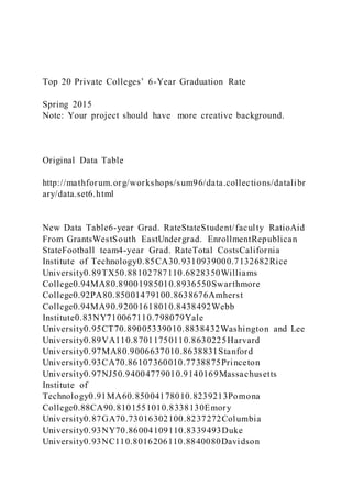
Top 20 Private Colleges’ 6-Year Graduation Rate
Spring 2015
Note: Your project should have more creative background.
Original Data Table
http://mathforum.org/workshops/sum96/data.collections/datalibr
ary/data.set6.html
New Data Table6-year Grad. RateStateStudent/faculty RatioAid
From GrantsWestSouth EastUndergrad. EnrollmentRepublican
StateFootball team4-year Grad. RateTotal CostsCalifornia
Institute of Technology0.85CA30.9310939000.7132682Rice
University0.89TX50.88102787110.6828350Williams
College0.94MA80.89001985010.8936550Swarthmore
College0.92PA80.85001479100.8638676Amherst
College0.94MA90.92001618010.8438492Webb
Institute0.83NY710067110.798079Yale
University0.95CT70.89005339010.8838432Washington and Lee
University0.89VA110.87011750110.8630225Harvard
University0.97MA80.9006637010.8638831Stanford
University0.93CA70.86107360010.7738875Princeton
University0.97NJ50.94004779010.9140169Massachusetts
Institute of
Technology0.91MA60.85004178010.8239213Pomona
College0.88CA90.8101551010.8338130Emory
University0.87GA70.73016302100.8237272Columbia
University0.93NY70.86004109110.8339493Duke
University0.93NC110.8016206110.8840080Davidson

College0.91NC100.82011645110.8934706Wellesley
College0.88MA90.88002300000.8437419Vassar
College0.87NY90.78002472100.8137870 Haverford
College0.92PA80.9001105100.8938928
Dependent variable
Independent variables
Independent
Binary
Independent
Categorical
Categorical Variables
Binary variables included: if the State
was majority Republican and if the school
had a football team. “0” or “1” representing
“no” or ”yes”.
Categorical variables include West, South West and North West.
North East will become my reference level.WestSouth
East1010000000000001001000001001000101000000
Reference level
The reference level selected was North East due to the fact the
North East region had the highest number of schools out of the
top 20. WestSouth
East1010000000000001001000001001000101000000
Depending on how you define regions in
the U.S. calculations on specific school
regions my differ. I kept it simple and only used key

regions relating to my data. Calculating all the regions
may cause the data to produce an error.
Removing 2 Variables due to Multicollinearty
I removed “Aid from Grants” because we already have “Total
Cost”. The amount of student aid paying for school doesn’t
really pertain when the table already gives the total cost of a 6-
year graduation rate.
I removed “4-year Grad. Rate” because this model gave us both
4-year and 6-year rates. Since we are looking for a 6-year rate
of graduation, they have already passed their 4-year
6
Keeping my variables
I left the States variable because its easier to read the model.
Also it helps relate my regions.
Student/faculty ratio was saved because it deals with real
numbers relating to how many students are on campus vs. how
many faculty members. In my opinion this is interesting and
important.
Undergraduate enrollment was left because it represents real
data of how many students are in the undergraduate enrollment.
Also I'm an undergraduate, so I can relate more to this data.
Total cost was left because I believe this variable is what
majority of students look at when choosing a college.
StateCATXMAPAMANYCTVAMACANJMACAGANYNCNCM
ANYPAStudent/faculty
Ratio35889771187569771110998Undergrad.
Enrollment9392787198514791618675339175066377360477941

7815516302410962061645230024721105Total
Costs326822835036550386763849280793843230225388313887
540169392133813037272394934008034706374193787038928
Lets Run It!
Alpha= 0.05
P-Value of Model=
0.0016
R= .8985
Adjusted R squared=
.6949
Adjusted R squared is used instead of R Square because dealing
with multiple regression, multiple variables calculated together
will cause inflation in the model.
69% of the variance can be explained by the model.
What is significant?
Alpha = 0.05
West has a p-value of 0.0318
Total Costs has a P-value of 0.0026
Football team
has a p-value of 0.0039

Outliers
The model did not have any outliers ( absence of outliers). All
variables had a reasonable p-value
The highest variable p-value was the “Republican State”, at
.7026 this is not enough to consider this variable an outlier.
If all the original variables were still included in my model,
then the number of outliers would have increased, but si nce I
shorted the list to only specific variables I thought pertained to
this model, I must of pulled out all possible outliers.
New model with only significant variables6-year Grad.
RateStateWestTotal CostsFootball teamCalifornia Institute of
Technology0.85CA1326820Rice
University0.89TX1283501Williams
College0.94MA0365501Swarthmore
College0.92PA0386760Amherst College0.94MA0384921Webb
Institute0.83NY080791Yale
University0.95CT0384321Washington and Lee
University0.89VA0302251Harvard
University0.97MA0388311Stanford
University0.93CA1388751Princeton
University0.97NJ0401691Massachusetts Institute of
Technology0.91MA0392131Pomona
College0.88CA1381301Emory
University0.87GA0372720Columbia
University0.93NY0394931Duke
University0.93NC0400801Davidson
College0.91NC0347061Wellesley
College0.88MA0374190Vassar

College0.87NY0378700Haverford
College0.92PA0389280binary varibalescategorical with 3
levelsindependent variablesdependent variable
I left the “States” variable because it
makes it easier to read the model and
there is no numerical value.
South East00000001000001011000Republican
State01010101000001111011Undergrad.
Enrollment9392787198514791618675339175066377360477941
7815516302410962061645230024721105Student/faculty
Ratio35889771187569771110998
Non-significant variables that were removed.
New model
Now lets run the model with significant levels only
Alpha= 0.05
R= .8590
Adjusted R squared= .6887
69% of the variance is explained
with this model
P-value= 0 or 6.5118E-05
Looks like “Total Cost” carries the best significant level (0)
according to this model.
Having a football team carries a p-value of 0.0008
Results of new model using only significant variables.

Using only significant variables changed how significant each
variable was.
At first, “West” had a p-value of 0.03179 and now it carries a p-
value of 0.0575. Not that much of a change but still a change.
“Total Cost” started at a p-value of 0.0026 and now it carries a
p-value of a value so small we consider it 0. Making “total
Cost” the most significant variable
Having a football team originally had a p-value of 0.0039 and
now carries a p-value of 0.0008.
Adjusted R squared = .6887 this number actually decreased
form original Adjusted R squared which was 0.6949. Not too far
off from the original, telling us that 68.8 or 69% of the variance
can be explained by this model.
Coefficients of new model
For every change in the X variable (independent variables), the
Y variable (independent variable) will change as well.
For total cost, the coefficient is 0.00000364. Since total coast is
calculated in $1000s, lets multiply the coefficient by 1000 and
you get a coefficient of 0.00364
It does look like having a football team will increase a 6-year
graduation rate by 4.3 %.
Total cost will increase the 6-year graduation rate by.36%
3 Predictions
My original data was out of 100 top private schools. For the
purpose of this model I only used the top 20. I will be using the
next three schools from my original table to make predictions.

Predictions will be based on my final table using only my
significant variables
Schools chosen: Northwestern University, Bowdoin College and
University of Pennsylvania
3 Predictions
Northwestern University
Has a football team which gives a value of “1” for “yes”
Lets call this region West which gives a value of “1” for “Yes”
Has a total cost of $38,817
Calculating my predictions I took the total cost and multiplied it
by the coefficient of the total cost.
38,817 x .000003643 = .141 or 14%
According to the original data the actual % was 92%, indicating
something is wrong with my variable units. Or this model is
bogus, but I would conclude that using data that carries several
different units such as % vs. $ amounts. Some conversions may
have to be re converted so all variables could be represented by
the same units.
The residual for this prediction was -78%
3 Predictions
Bowdoin College
Has a football team so they get a 1
Region located is North East which is my reference level so
they get a 0
Has a total cost of $38,663

Calculations
$38,663 x 0.000003643 = .1408 or 14%
Again my predictions are way off this has a residual of -76%
Original data indicated a 90%
3 Predictions
Prof. Decker Note: There are some issues with these
predictions. This project was used as an example because the
previous slides do such a good job clearly explaining variables
and the process of the project.
University of Pennsylvania
Has a football team so they get a 1
Located in the North East region so they get a 0
Total cost is $39,040
Calculating predictions:
39,040 x .000003643 = .142 or 14%
After looking at my predictions and the actual values I would
conclude some or all of my variables need to be converted into
the same unit of measurement. I would have to say some of the
values that were given m
PROJECT C:
· Read all documents in module
· Build data set with 1 Y dependent variable, 7 X independent
quantitative variables, 2 X independent binary variables, and 1
X independent categorical variable.
· Run the multiple regression test on the Full Dataset.

· Correct any error messages.
· use "2020 Directions for Multiple Regression Test" to run the
data and get to the Final Model
· Create Slides (Google version of PowerPoint) presentation
· Follow the step by step directions of "Project C Slides
Directions"
Directions for Running Multiple Regression Test 2020
How to Move/Copy individual Sheets in Excel:
In Excel, your entire project is called the Workbook, or Book
for short, and each tab in the Workbook is called a Spreadsheet,
or Sheet for short.
Any time you want to make a change/edit/delete to the project C
data set, rename and copy the individual Sheet you are working
on before you make the change, then make the changes to the
copy you just created. This ensures that you stay organized and
that every change you make is recorded.
To do this, right-click on “Sheet1” at the bottom of your Book,
then select “Rename” and name it something appropriate (Short
names are better). Next, right-click on your newly named tab
and select “Move or Copy…”. One here, you will click on the
checkbox at the bottom that says, “Create a copy” and select
where you want the copy to go, ( “(move to end)” is usually
best) and click “OK.” Repeat these steps every time you need
to make a change/edit/delete to the data.
Process 1: Building the Dataset

Use what you have learned from the video lessons, the 2020
Excel tips, as well as the advice from Professor Decker and
Emily to build your dataset. You will need 20 data points, 1 Y
dependent variable, and 10 X independent variables: 7
quantitative, 2 binary, 1 categorical (11 variables total). The
dataset with all 20 data points and 11 variables is called the
“Full Dataset.”
Tips for building the data set:
· Do not use a topic about sports.
· USE GOLDMINE
· If you choose counties for your 20 data points, pick ones with
populations over 80,000.
· The Y dependent variable is your most important decision, this
is what your entire project is about (try to pick something other
than population or area for this variable).
· Your 7 quantitative variables should be rates/percents (nothing
should be 0). However, please do not pick percent female or
male. Additionally, you can have the total population listed as a
quantitative variable (this will be the only total allowed).
· The binary variables answer a yes or no question, where 1=yes
and 0=no. Your chosen variable must have at least three 1’s and
at least three 0’s.
· The categorical variable also answers a yes or no question, but
these are broken into 3 groups with a reference level THAT IS
NEVER PART OF YOUR MODEL. The reference level is
chosen by you, just make sure you keep track of what you chose
and why.
· Please refer to “Multiple Regression Data Rules 2020” if you
have any other questions about the original dataset.
STOP NOW! EMAIL PROFESSOR DECKER AND EMILY!
YOU MUST GET YOUR DATASET APPROVED BEFORE
MOVING ON TO PROCESS 2!
Process 2: Seek and Destroy Collinear Variables

Collinear variables are two variables that are correlated, so they
should have a low p-value when they are run together in a
simple regression test. Even one pair of colinear variables will
ruin the study. Collinear variables must be avoided at all costs!
· Consider any
p-value less than 0.10 to indicate that the variables are
collinear.
An easy way to do this is start with
Independent X Variable 1 and use it to run a simple
regression test against another independent variable that you
think is collinear. For example,
Independent X Variable 2.
If the regression test’s p-value is less than 0.10, delete
one of the two independent x variables that you tested.
(REMEMBER, if you make any changes/edits/deletes
create a copy of your sheet!)
· Test at least 5 pairs of variables. Choose which pairs to test by
looking for any pairs that you think might have significant
correlation. However, if you have any reason to believe there
are other pairs of variables that correlate, test them too!
· The dataset after the collinear deletions is the “MC-free
dataset,” even if no deletions are made. MC-free stands for
multicollinearity-free because multicollinearity is a measure of
how collinear the variables are in a multiple regression test.
Your MC-free dataset must have at least 6 independent X
variables. If you have less than 6, add new variables, but test
them for being collinear to the old variables.

Process 3: Eliminating Insignificant Variables
· Run all the variables in the MC-free dataset in a multiple
regression correlation test and delete the variables with the
highest p-values until you have a total of 6 X variables
remaining (If you begin this process with 6 variables, move on
to the next bullet point).
· Next, run another multiple regression correlation test and
delete the variable with the highest p-value. This will leave you
with 5 X variables.
· Lastly, run one more multiple regression correlation test and
delete the variable with the highest p-value. This will leave you
with exactly 4 independent X variables (or your “Significant
Data Set”).
Process 4: Finding a Final Model
· A superior strategy for building a multiple regression model is
to test all possible combinations of variables and choose the
combination that has approximately the highest adjusted r2, but
fewest number of variables.
· This means that the best model has the highest adjusted r2 but
if two or more models have similar adjusted r2 numbers, then
choose the model with the least number of variables. If two
models have the exact same number of variables, then choose
the model with strictly the largest adjusted r2. (Adjusted r2
values are approximately the same if they are within 0.05).
Conduct 15 multiple regression tests; one test for each possible
combination of the four remaining independent variables (V1,
V2, V3, and V4). Below is all the possible combinations of
tests you need to do:

1. V1, V2, V3, V4
2. V1, V2, V3
3. V1, V2, V4
4. V1, V3, V4
5. V2, V3, V4
6. V1, V2
7. V1, V3
8. V1, V4
9. V2, V3
10. V2, V4
11. V3, V4
12. V1
13. V2
14. V3
15. V4
· Find the model with the highest adjusted r2 and any models
that have adjusted r2 within 0.05 of the highest one. From those
models, choose the one with the least number of variables. If
two models are tied for the least number of variables, choos e
the one with the highest r2 from those two.
· Your chosen model’s dataset is known as your “Final Model.”
Data
Rules for Multiple Regression – Set 4A for Project C
Excel analyzes a data set in multiple regression by dividing the
data into every possible combination of “boxes” (groups) based
on what levels the data points are in for qualitative variables
and the magnitude of their quantitative variables. It then
calculates what the value of the dependent variables would be
for each box. Problems arise when identical boxes are created
because it makes the independent variables dependent on each
other resulting in collinear variables.

Violating these rules will cause an error message in the p-value
on your analysis print out. One error message will ruin your
project! Contact the professor for help immediately if you
cannot fix an error message in your print out.
The examples are for a model of real estate where the dependent
variable is the price of the homes.
Rule #1: Data points may not have a value of zero for
quantitative variables.
Reason and
Solution
: Zero is a very low number when compared to the values of the
other data points. This makes data points with zeros major
outliers. The outlier will ruin the calculation. If only one of
your data points is zero, remove it as an outlier. If you have
several zeros, convert the quantitative variable to a qualitative
variable by coding the data points that have values that are not
zero as “1” and the data points that have values that are zero as
“0.”
Example: If some homes have an HOA fee of a few hundred
dollars and some homes do not have an HOA so there is no
HOA fee, make this variable qualitative by having homes with

HOA fees coded as “1” and homes without HOA fees coded as
“0” instead of entering the HOA fees as their quantitative
numbers where homes without HOA fees entered as zeros.
Rule #2: Quantitative variables for rates cannot be complements
or each other (add to 100%) and one quantitative variable
cannot be determined by an algorithm (formula) of other
quantitative variables.
Reason and

Top 20 Private Colleges’ 6-Year Graduation RateSpring 2015

Recommended

Recommended

More Related Content

Similar to Top 20 Private Colleges’ 6-Year Graduation RateSpring 2015

Similar to Top 20 Private Colleges’ 6-Year Graduation RateSpring 2015 (20)

More from AnastaciaShadelb

More from AnastaciaShadelb (20)

Recently uploaded

Recently uploaded (20)

Top 20 Private Colleges’ 6-Year Graduation RateSpring 2015