1. 1
Andrew Rogala STAT 481 Student Project
ResearchGoal and Data:
The goal of the analysis is to develop a statistical model to predict default status (Yes, No) of
credit card customers given the predictors income, balance, and student status (Yes, No).
Additionally, it would be advantageous to take the view point of a credit card company and
produce a model with a high true positive rate, a low false positive rate, and a high detection rate.
To accomplish this a low probability threshold is needed. The data used for this analysis is the
Default data set in the ISLR library. It is a simulated data set containing information on ten
thousand customers.
Response Variable:
The response variable is default status Yes or No.
Predictor Variables:
The predictor variables are annual income in dollars, average balance, in dollars, that the
customer has remaining on their credit card after making their monthly payment, and student
status Yes or No.
Statistical Methods:
Multiple logistic regression and the validation set approach will be used. The validation set
approach will gauge how well the model will perform on a new set of data.
Summary Statistics for the Default data set:
default student balance income
No : 9667 No : 7056 Min. : 0.0 Min. : 772
Yes: 333 Yes: 2944 1st Qu. : 481.7 1st Qu. : 21340
Median : 823.6 Median : 34553
Mean : 835.4 Mean : 33517
3rd Qu. : 1166.3 3rd Qu. : 43808
Max. : 2654.3 Max. : 73554
P(default = Yes) = 333/10,000 = 0.0333
P(default = No) = 9667/10,000 = 0.9667
(student)
No Yes
(default) No 6850 2817
Yes 206 127
P(default = Yes given student = Yes) = 127/(2817+127) = 0.04313859
P(default = Yes given student = No) = 206/(6850+206) = 0.02919501
2. 2
Student = red Plot taken from “An Introduction to Statistical Learning” page 137
Non-Student = blue
Box Plots:
From the left box plot below it appears that those individuals who defaulted tended to have much
higher credit card balances. This solid relationship between the predictor variable balance and
the response variable default suggests there is a strong correlation between the two of them.
From the right box plot below it appears that those individuals who defaulted tended to have a
slightly lower median income. Thus, the predictor income is slightly correlated with the response
default. Next, I will plot box plots for student and balance as well as student and income to see if
there is any collinearity between these predictor variables.
No Yes
05001000150020002500
Default
CreditCardBalance
No Yes
0200004000060000
Default
Income
3. 3
Analysis of the left boxplot below shows that students tend to have slightly higher credit card
balances than non-students and thus student and balance are correlated. Analysis of the right
boxplot below shows that students tend to have much lower incomes than non-students; thus the
student and income variables are correlated. Due to the collinearity between these predictor
variables I will initially leave the student variable out of the logistic regression and just fit a
model for default with income and balance as predictors. Later I will add all three and see which
model produces better results.
The 1st fit model on the training data is:
𝑙𝑜𝑔(
𝑝( 𝑑𝑒𝑓𝑎𝑢𝑙𝑡)
1−𝑝( 𝑑𝑒𝑓𝑎𝑢𝑙𝑡)
) = -11.27 + 0.00001788(income) + 0.005538(balance)
P(default) =
1
1+𝑒−(−11.27+0.00001788( 𝑖𝑛𝑐𝑜𝑚𝑒)+0.005538(𝑏𝑎𝑙𝑎𝑛𝑐𝑒))
P-value for income = 0.0117
P-value for balance < 2 x 10-16
Thus both income and balance are significant predictors of default
No Yes
05001000150020002500
Student Status
CreditCardBalance
No Yes
0200004000060000
Student Status
Income
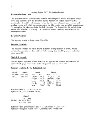
4. 4
Area under the curve = 0.9493
Probability threshold = 0.03540053
Confusion Matrix and Statistics
(Observed)
No Yes
(Predicted) No 4188 17
Yes 644 151
% Correctly Classified = Accuracy = 0.8678
True Positive Rate = Sensitivity = 0.8988 P(predict default/default)
True Negative Rate = Specificity = 0.8667 P(predict not default/ not default)
False Positive Rate = (1 - Specificity) = 0.1333
Prevalence = 0.0336
Detection Rate = 151/5000 = 0.0302
Detection Prevalence = (644+151)/5000 = 0.1590
%Misclassified = Test Error = (644+17)/5000 = 0.1322 = 13.22%
The 2nd fit model on the training data is:
𝑙𝑜𝑔(
𝑝( 𝑑𝑒𝑓𝑎𝑢𝑙𝑡)
1−𝑝( 𝑑𝑒𝑓𝑎𝑢𝑙𝑡)
) = -10.64 + 0.000001296(income) + 0.005615(balance) + -0.5947(student)
P(default) =
1
1+𝑒−(−10.64+0.000001296( 𝑖𝑛𝑐𝑜𝑚𝑒)+0.005615( 𝑏𝑎𝑙𝑎𝑛𝑐𝑒)+ −0.5947(𝑠𝑡𝑢𝑑𝑒𝑛𝑡))
ROC Curve 1st model
False positive rate
Truepositiverate
0.0 0.2 0.4 0.6 0.8 1.0
0.00.20.40.60.81.0
5. 5
P-value for income = 0.9112
P-value for balance < 2 x 10-16
P-value for student = 0.0708
Thus balance is the only significant predictor of default in this model. However, depending on
the choice of alpha student may be considered a significant predictor as well.
Area under the curve = 0.9503
Probability threshold = 0.03197311
Confusion Matrix and Statistics
(Observed)
No Yes
(Predicted) No 4160 16
Yes 672 152
% Correctly Classified = Accuracy = 0.8624
True Positive Rate = Sensitivity = 0.9048 P(predict default/default)
True Negative Rate = Specificity = 0.8609 P(predict not default/ not default)
False Positive Rate = (1 - Specificity) = 0.1391
Prevalence = 0.0336
Detection Rate = 152/5000 = 0.0304
Detection Prevalence =(672+152)/5000 = 0.1648
%Misclassified = Test Error = (672+16)/5000 = 0.1376 = 13.76%
ROC Curve 2nd model
False positive rate
Truepositiverate
0.0 0.2 0.4 0.6 0.8 1.0
0.00.20.40.60.81.0
6. 6
Interpretation of Results:
Overall, without taking income and balance into consideration students have a higher
probability of default (0.0431) as compared to the probability of default for non-students
(0.0292). Thus, if nothing is known about a customer’s income or credit card balance students
are a risker population. However, by examining the graph on page two it is clear that students
(red) with the same balance as non-students (blue) have a lower default rate than non-students.
The correlation between student and balance explains this paradox. Students tend to have higher
credit card balances than non-students, see box plot on page three, and it is known that customers
with higher balances are more likely to default; see box plot on page two. Even though the
student population is more likely to have higher credit card balances, which tend to be associated
with higher default rates, it is still possible for an individual student to have a lower probability
of default than a non-student given that they have the same income and balance. The conclusion
is that if no information is given about a customer’s balance and income students are risker;
however, a student is less risky than a non-student with the same balance and income.
The first model has a slightly smaller test error of 13.22%, as opposed to the second
model’s test error of 13.76%. In addition, the first model produced better p-values for its
predictors. However, with the addition of the student variable, the second model provides
significantly more information to justify using this model as the main method for predicting
default.
The second model has an area under the ROC curve of 0.9503 suggesting a good fit. It
also has a high true positive rate (0.9048), a reasonable false positive rate of (0.1391), a high
detection rate of 0.0304, and a test error of 13.76%. Also out of 5000 predictions only 16 were
predicted to be No and observed to be a Yes. In theory, using this model a credit card company
could reduce their default rate to 16/5000 = 0.32% as compared to the observed default rate of
3.36%.
By choosing a small probability threshold a high true positive rate was achieved, however
doing this does cause the test error to increase. A sacrifice worthwhile taking the view of a credit
card company trying to reduce their default rate. The threshold can be changed to modify this
model to fit the specific needs of users.
Now an interpretation of the second model is a follows. A one unit increase in balance is
associated with an increase in the log odds of default by 0.005615 units when holding all other
predictors constant. A one unit increase in income is associated with an increase in the log odds
of default by 0.000001296 units when holding all other predictors constant. Finally, a student is
associated with a decrease in default by 0.5947 units when holding all other predictors constant.
7. 7
R Code and R OutPut:
>library(pROC)
>library(ROCR)
>library(mgcv)
>library(caret)
>library(e1071)
>library(ISLR)
> attach(Default)
> fix(Default)
> dim(Default)
[1] 10000 4
> ?Default
> summary(Default)
default student balance income
No :9667 No :7056 Min. : 0.0 Min. : 772
Yes: 333 Yes:2944 1st Qu.: 481.7 1st Qu.:21340
Median : 823.6 Median :34553
Mean : 835.4 Mean :33517
3rd Qu.:1166.3 3rd Qu.:43808
Max. :2654.3 Max. :73554
> #P(Default = Yes)
> 333/10000
[1] 0.0333
> #P(Default = No)
> 9667/10000
[1] 0.9667
> #Some Conditional Probabilities
> table(Default$default,Default$student)
No Yes
No 6850 2817
Yes 206 127
> #P(default = Yes given student = Yes)
> 127/(2817+127)
[1] 0.04313859
> #P(default = Yes given student = No)
> 206/(6850+206)
[1] 0.02919501
>#Box Plots
> par(mfrow=c(1,2))
> plot(default, balance, xlab="Default", ylab="Credit Card Balance", col="red")
> plot(default, income, xlab="Default", ylab="Income", col="green")
> par(mfrow=c(1,2))
8. 8
> plot(student,balance,xlab="Student Status",ylab="Credit Card Balance", col="red")
> plot(student,income,xlab="Student Status",ylab="Income", col="green")
> #Training and HoldOut Sets
> set.seed(23)
> ReSampleData = Default[sample(nrow(Default)),]
> Data.Set.Splits = cut(seq(1,nrow(ReSampleData)),breaks=2,labels=FALSE)
> tIndexes = which(Data.Set.Splits!=1,arr.ind=TRUE)
> Training.Set = ReSampleData[tIndexes, ]
> fix(Training.Set)
> HoldOut.Set = ReSampleData[-tIndexes,]
> fix(HoldOut.Set)
> #fit the 1st logistic regression on training data
> default.glm.training = glm(default~income + balance,
family=binomial(link="logit"),data=Training.Set)
> summary(default.glm.training)
Call:
glm(formula = default ~ income + balance, family = binomial(link = "logit"),
data = Training.Set)
Deviance Residuals:
Min 1Q Median 3Q Max
-2.4201 -0.1489 -0.0604 -0.0231 3.6961
Coefficients:
Estimate Std. Error z value Pr(>|z|)
(Intercept) -1.127e+01 6.000e-01 -18.778 <2e-16 ***
income 1.788e-05 7.088e-06 2.522 0.0117 *
balance 5.538e-03 3.162e-04 17.516 <2e-16 ***
---
Signif. codes: 0 ‘***’ 0.001 ‘**’ 0.01 ‘*’ 0.05 ‘.’ 0.1 ‘ ’ 1
(Dispersion parameter for binomial family taken to be 1)
Null deviance: 1450.21 on 4999 degrees of freedom
Residual deviance: 797.18 on 4997 degrees of freedom
AIC: 803.18
Number of Fisher Scoring iterations: 8
> #predicts probabilities for holdout set values using the training set model
> HoldOut.Set$predict.default.glm.hold=predict(default.glm.training,
type="response",newdata=data.frame(HoldOut.Set))
> fix(HoldOut.Set)