Help with MATLAB Assignments, homework, projects only @ http://Allassignmentexperts.com

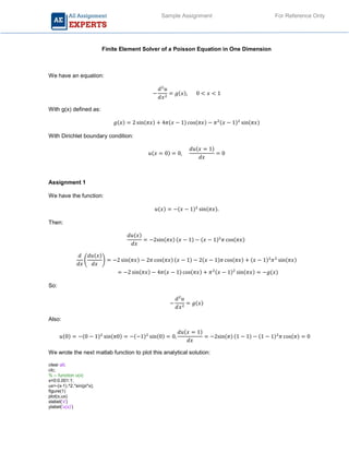
1. Sample Assignment For Reference Only
Finite Element Solver of a Poisson Equation in One Dimension
We have an equation:
, 0 1
With g(x) defined as:
2 sin 4 1 cos 1 sin
With Dirichlet boundary condition:
0 0,
1
0
Assignment 1
We have the function:
1 sin .
Then:
2sin 1 1 cos
2 sin 2 cos 1 2 1 cos 1 sin
2 sin 4 1 cos 1 sin
So:
Also:
0 0 1 sin 0 1 sin 0 0,
1
2sin 1 1 1 1 cos 0
We wrote the next matlab function to plot this analytical solution:
clear all;
clc;
% -- function u(x)
x=0:0.001:1;
ux=-(x-1).^2.*sin(pi*x);
figure(1)
plot(x,ux)
xlabel('x')
ylabel('u(x)')

2. Sample Assignment For Reference Only
And here is the figure for u(x)
Assignment 2.
Here, we can write the numerical scheme to get the algorithm for numerical solution of our equation.
We know, that the second derivative at some point i can be represented as next:
2
∆
Thus, we can write en equation of form:
1; 2; 1
2∆
∗ ∆
So, as we see we can write the next equation:
Where:
- A is tridiagonal matrix (non-zero elements only on main diagonal and on elements up and beneath from
it).
- u is unknown vector of function we looking at.
- g is a vector with function g(x) values at points xi.
Assignment 3.
The trapezoidal rule can be written is the next way :
2

3. Sample Assignment For Reference Only
We can write the our intermediate matrix Sei which appear for every step and every element ei as the next
(here we use the result for matrix A from previous part):
1 1 1
1 1
Using previous part and trapezoidal rule we can write the vector fei as the next:
2
Assignment 4.
The next step will be to assemble all our element matrixes Sei in one global matrices, for example if we only
have 2 nodes in our system we can assemble matrices Se1 and Se2 in the next way:
1 1 1
1 1
,
1 1 1
1 1
, ,
1/ 1/ 0
1/ 1/ 1/ 1/
0 1/ 1/
So, we see that for N=2 nodes we have 3x3 matrix , this will work also in the general case when we have N
nodes and (N+1)x(N+1) global matrix.
The same induction we can build for vector fei, for example for 2 nodes we will have:
2
,
2
,
2
2
Assignment 5.
This was done as additional function in Matlab:
function f=GenerateMesh(xo,xe,N)
% --- create the mesh of N+1 point in range x0 ... xe
dx=(xe-xo)/N;
for i=1:N+1
x(i)=xo+dx*(i-1);
end
f=x;
end
Assignment 6.
This was done as additional function in Matlab:
function f=SourceFct(xi)
% -- gives value of source function at xi
f=2*sin(pi*xi)+4*pi*(xi-1)*cos(pi*xi)-pi^2*(xi-1)^2*sin(pi*xi);
end
Assignment 7.

4. Sample Assignment For Reference Only
This was done as additional function in Matlab:
function f=GenerateTopology(N)
% -- generate topology matrix
f=zeros(N,2);
for i=1:N
f(i,1)=i;
f(i,2)=i+1;
end
end
Assignment 8.
This was done as additional function in Matlab:
function f=GenerateElementMatrix(xi,xi1)
% -- input , the values of x(i) and x(i+1)
Sei=[1 -1; -1 1];
Sei=Sei/(xi1-xi);
f=Sei;
end
Assignment 9.
This was done as additional function in Matlab:
function f=GenerateElementVector(xi,xi1)
gi=SourceFct(xi);
gi1=SourceFct(xi1);
f=[gi*(xi1-xi)/2;gi1*(xi1-xi)/2];
end
Assignment 10.
This was done as additional function in Matlab:
function f=AssembleMatrix(xo,xe,N)
S=zeros(N+1,N+1);
x=GenerateMesh(xo,xe,N);
elmat=GenerateTopology(N);
for i=1:N
Sei=GenerateElementMatrix(x(i),x(i+1));
for j=1:2
for k=1:2
S(elmat(i,j),elmat(i,k))=S(elmat(i,j),elmat(i,k))+Sei(j,k);
end
end
end
f=S;
end
Assignment 11.
This was done as additional function in Matlab:
function f=AssembleVector(xo,xe,N)
fv=zeros(N+1,1);
x=GenerateMesh(xo,xe,N);
elmat=GenerateTopology(N);
for i=1:N
fei=GenerateElementVector(x(i),x(i+1));

5. Sample Assignment For Reference Only
for j=1:2
fv(elmat(i,j))=fv(elmat(i,j))+fei(j);
end
end
f=fv;
end
Assignment 12.
This was reached by adding next lines to main program when we calculate the matrix S and vector f before
use them to solve en equation :
% boundary ---
S(1,1)=1;
S(1,2)=0;
f(1)=0;
Assignment 13.
We run our main program for N=100 and got the next visualization for S matrix as
Assignment 14.
Here is the graphs where we have two solutions, analytical u(x) from first part and numerical for N=8, and
N=32.
N=8 N=32

6. Sample Assignment For Reference Only
As we see – for more number of nodes we have better convergence between two solutions, analytical and
numerical.
Elective Part
Part 1
Lets try to write analytical solution as:
1 sin 2
This will give the same result for second derivative as we know that 2 0
So, we after changes in main and additional function we will get the result.
As we see the results very unclose – this can be explained that we need change not only analytical solution
but also the boundary conditions.
Part 2
To compare results for different number of nodes we can write the loop for different N=2,4,8,16,… etc. On
every loop we calculate the numerical solution and the error (largest values for mesh).

7. Sample Assignment For Reference Only
And we got the next graph for norm of error vs. number of nodes (see q_err.m file):
As we see , in logarithmic axes we have linear dependence for logarithm of norm of error from logarithm from
number of nodes, this leads from the way we wrote our equations using linear (first order) Lagrangian shape
functions.
Part 3
Here we changed the program by adding to last element in vector f the value:
, 1/
So, in this way we got the next graph with different numerical solutions (for N=16) for different values of α
(see q_neumann.m for script):
As we see – with increasing of α we get the increasing of left boundary of function