MACHINE LEARNING IS GOING TO DEFINE THE NEXT ERA; PEOPLE SAY IT WILL HAVE SIMILAR EFFECTS AS ELECTRICITY OR INTERNET HAD IN their TIMES .ARITIFICIAL INTELLIGENCE IS THE NEXT BEST THING IN THE WORLD OF TECHNOLOGY , BLOCKCHAIN AFTER THAT

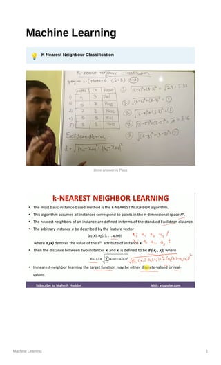
1. Machine Learning 1
Machine Learning
💡 K Nearest Neighbour Classification
Here answer is Pass

2. Machine Learning 2

3. Machine Learning 3

4. Machine Learning 4

5. Machine Learning 5
💡 Weighted KNN
Final answer is False

6. Machine Learning 6

7. Machine Learning 7
💡 K means Clustering

8. Machine Learning 8
v

9. Machine Learning 9
💡 Principal Component Analysis
It Reduces overfitting problem
It reduces dimension (Features) to solve problem of overfitting
Number of Principle component can be less than or equal to Number of features
PC1 will have highest Priority
All Principle components should be independent
Example➖
Steps
Find mean
Find covarainace matrix

10. Machine Learning 10
Steps➖
Find Eigen Values Lambda1 and Lambda2
For each eigen value , find eigen vector
This 2 eigen vectors are our final answer

11. Machine Learning 11
PRACTICE PROBLEMS BASED ON PRINCIPAL
COMPONENT ANALYSIS-
Consider the two dimensional patterns (2,
1), (3, 5), (4, 3), (5, 6), (6, 7), (7, 8). Compute
the principal component using PCA
Algorithm.
Solution-
We use the above discussed PCA Algorithm-
Step-01:
Get data.
The given feature vectors are-
x = (2, 1)
1
x = (3, 5)
2
x = (4, 3)
3

12. Machine Learning 12
x = (5, 6)
4
x = (6, 7)
5
x = (7, 8)
6
Step-02:
Calculate the mean vector (µ).
Mean vector (µ)
= ((2 + 3 + 4 + 5 + 6 + 7) / 6, (1 + 5 + 3 + 6 + 7 + 8) / 6)
= (4.5, 5)
Thus,
Step-03:
Subtract mean vector (µ) from the given feature vectors.
x – µ = (2 – 4.5, 1 – 5) = (-2.5, -4)
1
x – µ = (3 – 4.5, 5 – 5) = (-1.5, 0)
2
x – µ = (4 – 4.5, 3 – 5) = (-0.5, -2)
3
x – µ = (5 – 4.5, 6 – 5) = (0.5, 1)
4
x – µ = (6 – 4.5, 7 – 5) = (1.5, 2)
5
x – µ = (7 – 4.5, 8 – 5) = (2.5, 3)
6
Feature vectors (xi) after subtracting mean vector (µ) are-
Step-04:
Calculate the covariance matrix.
Covariance matrix is given by-

13. Machine Learning 13
Now,
Now,
Covariance matrix
= (m1 + m2 + m3 + m4 + m5 + m6) / 6
On adding the above matrices and dividing by 6, we get-
Step-05:
Calculate the eigen values and eigen vectors of the covariance matrix.
λ is an eigen value for a matrix M if it is a solution of the characteristic equation |M – λI|
= 0.
So, we have-
From here,
(2.92 – λ)(5.67 – λ) – (3.67 x 3.67) = 0
16.56 – 2.92λ – 5.67λ + λ2 – 13.47 = 0
λ2 – 8.59λ + 3.09 = 0
Solving this quadratic equation, we get λ = 8.22, 0.38
Thus, two eigen values are λ1 = 8.22 and λ2 = 0.38.
Clearly, the second eigen value is very small compared to the first eigen value.

14. Machine Learning 14
So, the second eigen vector can be left out.
Eigen vector corresponding to the greatest eigen value is the principal component for
the given data set.
So. we find the eigen vector corresponding to eigen value λ1.
We use the following equation to find the eigen vector-
MX = λX
where-
M = Covariance Matrix
X = Eigen vector
λ = Eigen value
Substituting the values in the above equation, we get-
Solving these, we get-
2.92X1 + 3.67X2 = 8.22X1
3.67X1 + 5.67X2 = 8.22X2
On simplification, we get-
5.3X1 = 3.67X2 ………(1)
3.67X1 = 2.55X2 ………(2)
From (1) and (2), X1 = 0.69X2
From (2), the eigen vector is-
Thus, principal component for the given data set is-
Lastly, we project the data points onto the new subspace as-

15. Machine Learning 15
💡 Conditional Probability & Bayes Theorem

16. Machine Learning 16
💡 Naive Bayes Classifier
Answer is banana

17. Machine Learning 17

18. Machine Learning 18

19. Machine Learning 19

20. Machine Learning 20
B is the winner

21. Machine Learning 21

22. Machine Learning 22

23. Machine Learning 23

24. Machine Learning 24

25. Machine Learning 25
💡 Logistic Regression

26. Machine Learning 26

27. SUPPORT VECTOR MACHINE

30. ENDS

31. ENTROPY OF TRUE EXAMPLE

37. ID3 Decision tree Learning Algorithm

38. • EXAMPLE-1
WHOLE ENTROPY
ATTRIBUTE WITH MAX INFO GAIN IS ROOT NODE

44. • EAXMPLE – 2

46. ENSEMBLE TECHNIQUE
In statistics and machine learning, ensemble methods use multiple learning algorithms to obtain
better predictive performance than could be obtained from any of the constituent learning
algorithms alone.

47. https://www.youtube.com/watch?v=nxFG5xdpDto&list=PLZoTAELRM
XVPBTrWtJkn3wWQxZkmTXGwe&index=64
https://www.youtube.com/watch?v=NLRO1-
jp5F8&list=PLZoTAELRMXVPBTrWtJkn3wWQxZkmTXGwe&index=68

49. t – target output
o – obtained output

50. https://www.youtube.com/watch?v=dM_8Y41EgsY&list=PL4gu8xQu0_5JBO1FKRO5p20wc8DprlOgn&ind
ex=58

53. Hidden layer

54. EXAMPLE - 1

56. https://www.youtube.com/watch?v=AWhboi1aTxI&list=PL4gu8xQ
u0_5JBO1FKRO5p20wc8DprlOgn&index=67

57. CNN
• https://www.youtube.com/watch?v=cleLMnmNMpY
• https://www.youtube.com/watch?v=Etksi-
F5ug8&t=1s
• https://www.youtube.com/watch?v=PGBop7Ka9AU&
t=9s
• https://www.youtube.com/watch?v=aLjpU-ahEhA
• https://www.youtube.com/watch?v=VpSLtKiPhLM
• Solved example:-
https://www.youtube.com/watch?v=AN9sZUFyxCo