The document describes material balance calculations and the Tracy method for predicting future reservoir performance. It presents the general material balance equation and shows how it can be rearranged and solved to determine oil initially in place (OOIP), drive mechanisms, and future production based on phi factors. The Tracy method uses the material balance equation and phi factors calculated from reservoir fluid properties to generate tables and plots predicting cumulative oil, gas, and gas-oil ratio at future reservoir pressures.

1. 1
( ) ( ) ( )
( ) B
W
+
B
R
-
R
N
+
B
N
=
B
G
+
B
W
+
W
+
p
S
-
1
S
C
+
C
GB
+
NB
+
B
-
B
G
+
B
-
B
N
w
p
g
soi
p
p
t
p
Ig
I
Iw
I
e
t
wi
wi
w
f
gi
ti
gi
g
ti
t ∆






Material Balance Calculations
A general material balance equation that can be applied to all reservoir types was
first developed by Schilthuis in 1936. Although it is a tank model equation, it can
provide great insight for the practicing reservoir engineer. It is written from start of
production to any time (t) as follows:
oil zone oil expansion + gas zone gas expansion
+ oil zone and gas zone pore volume and connate water expansion
+ water influx + water injected + gas injected
= oil produced + gas produced + water produced
Where:
N initial oil in place, STB
Np cumulative oil produced, STB
G initial gas in place, SCF
GI cumulative gas injected into reservoir, SCF
Gp cumulative gas produced, SCF
We water influx into reservoir, bbl
WI cumulative water injected into reservoir, STB
Wp cumulative water produced, STB
Bti initial two-phase formation volume factor, bbl/STB = Boi
Boi initial oil formation volume factor, bbl/STB
Bgi initial gas formation volume factor, bbl/SCF
Bt two-phase formation volume factor, bbl/STB = Bo + (Rsoi - Rso) Bg
Bo oil formation volume factor, bbl/STB
Bg gas formation volume factor, bbl/SCF
Bw water formation volume factor, bbl/STB
BIg injected gas formation volume factor, bbl/SCF
BIw injected water formation volume factor, bbl/STB
Rsoi initial solution gas-oil ratio, SCF/STB
Rso solution gas-oil ratio, SCF/STB
Rp cumulative produced gas-oil ratio, SCF/STB
Cf formation compressibility, psia-1
Cw water isothermal compressibility, psia-1
Swi initial water saturation
∆pt reservoir pressure drop, psia = pi - p(t)
p(t) current reservoir pressure, psia
(1)

2. 2
( ) ( ) ( )
( ) B
W
+
B
R
-
R
N
+
B
N
=
B
G
+
B
W
+
W
+
p
S
-
1
S
C
+
C
GB
+
NB
+
B
-
B
G
+
B
-
B
N
w
p
g
soi
p
p
t
p
Ig
I
Iw
I
e
t
wi
wi
w
f
gi
ti
gi
g
ti
t ∆






B
N
B
G
=
volume
oil
initial
volume
cap
gas
initial
ti
gi
=
m
( ) ( ) ( )
( ) B
W
+
B
R
-
R
N
+
B
N
=
B
G
+
B
W
+
W
+
p
S
-
1
S
C
+
C
B
Nm
+
NB
+
B
-
B
B
B
Nm
+
B
-
B
N
w
p
g
soi
p
p
t
p
Ig
I
Iw
I
e
t
wi
wi
w
f
ti
ti
gi
g
gi
ti
ti
t ∆






Material Balance Equation as a Straight Line
Normally, when using the material balance equation, each pressure and the
corresponding production data is considered as being a separate point from other pressure
values. From each separate point, a calculation is made and the results of these
calculations are averaged.
However, a method is required to make use of all data points with the
requirement that these points must yield solutions to the material balance equation that
behave linearly to obtain values of the independent variable. The straight-line method
begins with the material balance written as:
Defining the ratio of the initial gas cap volume to the initial oil volume as:
and plugging into the equation yields:
Let:

3. 3
( )
[ ] B
G
-
B
W
-
B
W
+
B
R
-
R
+
B
N
=
F
p
S
-
1
S
C
+
C
=
E
B
-
B
=
E
B
-
B
=
E
Ig
I
Iw
I
w
p
g
soi
p
t
p
t
wi
wi
w
f
w
f,
gi
g
g
ti
t
o
∆






( )
( ) W
+
E
B
m
+
1
+
E
B
B
m
+
E
N
=
W
+
E
B
m
+
1
N
+
E
B
B
Nm
+
E
N
=
F
e
w
f,
ti
g
gi
ti
o
e
w
f,
ti
g
gi
ti
o






( ) 





E
B
m
+
1
+
E
B
B
m
+
E
=
D w
f,
ti
g
gi
ti
o
D
W
+
N
=
D
F e
Thus we obtain:
Let:
Dividing through by D, we get:
Which is written as y = b + x. This would suggest that a plot of F/D as the y coordinate
and We/D as the x coordinate would yield a straight line with slope equal to 1 and
intercept equal to N.
(2)

4. 4
Drive Indexes from the Material Balance Equation
The three major driving mechanisms are: 1) depletion drive (oil zone oil
expansion), 2) segregation drive (gas zone gas expansion), and 3) water drive (water
zone water influx). To determine the relative magnitude of each of these driving
mechanisms, the compressibility term in the material balance equation is neglected and
the equation is rearranged as follows:
Dividing through by the right hand side of the equation yields:
The terms on the left hand side of equation (3) represent the depletion drive index (DDI),
the segregation drive index (SDI), and the water drive index (WDI) respectively. Thus,
using Pirson's abbreviations, we write:
DDI + SDI + WDI = 1
( ) ( ) ( ) ( )
[ ]
B
R
-
R
+
B
N
=
B
W
-
W
+
B
-
B
G
+
B
-
B
N g
soi
p
t
p
w
p
e
gi
g
ti
t
( )
( )
[ ]
( )
( )
[ ]
( )
( )
[ ]
1
=
B
R
-
R
+
B
N
B
W
-
W
+
B
R
-
R
+
B
N
B
-
B
G
+
B
R
-
R
+
B
N
B
-
B
N
g
soi
p
t
p
w
p
e
g
soi
p
t
p
gi
g
g
soi
p
t
p
ti
t
(3)

5. 5
Tracy Material Balance
Tracy started with the Schilthuis form of the material balance equation:
Since:
Plugging into the equation, rearranging, and solving for N yields:
Let:
( ) ( ) ( ) w
p
g
soi
p
p
t
p
e
gi
g
ti
t B
W
B
R
-
R
N
+
B
N
=
W
B
-
B
G
+
B
-
B
N +
+
( )B
R
-
R
+
B
=
B
B
=
B
R
N
=
G
B
B
Nm
=
G
g
so
soi
o
t
oi
ti
p
p
p
gi
ti
[ ]
( ) ( )





−
−
B
-
B
B
B
m
+
B
R
-
R
+
B
-
B
B
W
W
B
G
+
B
R
-
B
N
=
N
gi
g
gi
oi
g
so
soi
oi
o
w
p
e
g
p
g
so
o
p )
(
( ) ( ) ( )
( ) ( ) ( )
( ) ( ) ( )





Φ






Φ






Φ
B
-
B
B
B
m
+
B
R
-
R
+
B
-
B
=
B
-
B
B
B
m
+
B
R
-
R
+
B
-
B
B
=
B
-
B
B
B
m
+
B
R
-
R
+
B
-
B
B
R
-
B
=
gi
g
gi
oi
g
so
soi
oi
o
W
gi
g
gi
oi
g
so
soi
oi
o
g
G
gi
g
gi
oi
g
so
soi
oi
o
g
so
o
N
1

6. 6
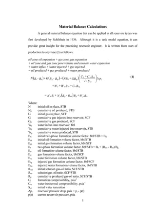
Phi vs Reservoir Pressure
0.01
0.1
1
10
100
0 500 1000 1500 2000
Reservoir Pressure, psia
P
ressu
re
F
acto
r
phiG
phiW
PhiN vs Reservoir Pressure
0
5
10
15
20
25
30
35
40
0 500 1000 1500 2000
Reservoir Pressure, psia
Pre
s
s
u
re
F
a
c
to
r
phiN
Thus we have:
If there is no water influx or water production, the equation is written as:
Φ
Φ G
p
N
p G
+
N
=
N
Phi factors can be calculated at all desired pressures using data from a reservoir fluid
analysis. Then a table or plot of these factors can be used to calculate oil in place or
predict future performance.
Phi factors are infinite at the bubble point and decline rapidly as pressure declines below
the bubble point. Characteristic shapes of these pressure functions are shown next.
( )Φ
−
+
Φ
Φ W
e
w
p
G
p
N
p W
B
W
G
+
N
=
N

7. 7
Tracy Method for Predicting Future Performance
For oil reservoirs above the bubble-point pressure, the Tracy prediction method is
not needed. It is normally started at the bubble-point pressure or at pressures below. To
use this method for predicting future performance, it is necessary to choose the future
pressures at which performance is desired. This means that we need to select the pressure
step to be used. At each selected pressure, cumulative oil, cumulative gas, and producing
gas-oil ratio will be calculated. So the goal is to determine a table of Np, Gp, and Rp
versus future reservoir static pressure such as:
n p Np Gp Rp
0
1
2
3
4
p0 = pi = pb
p1
p1
p3
p4
0
Np1
Np2
Np3
Np4
0
Gp1
Gp2
Gp3
Gp4
Rsb
R1
R2
R3
R4
Oil is produced from volumetric, undersaturated reservoirs by the expansion of reservoir
fluids. Down to the bubble-point pressure, the production is caused by liquid (oil and
connate water) expansion and rock compressibility. Below the bubble-point pressure, the
expansion of the connate water and the rock compressibility are negligible, and as the oil
phase contracts owing to release of gas from solution, production is a result of expansion
of the gas phase. As production proceeds, pressure drops and the gas and oil viscosities
and volume factors continually change.
Tracy method for predicting the performance of internal gas drive reservoir uses
the material balance equation for a volumetric undersaturated oil reservoir which is
written as:
( ) ( ) ( ) w
p
g
soi
p
p
t
p
e
gi
g
ti
t B
W
B
R
-
R
N
+
B
N
=
W
B
-
B
G
+
B
-
B
N +
+

8. 8
Since:
Plugging into the equation, rearranging, and solving for N yields:
Let:
Thus we have:
( )B
R
-
R
+
B
=
B
B
=
B
R
N
=
G
B
B
Nm
=
G
g
so
soi
o
t
oi
ti
p
p
p
gi
ti
[ ]
( ) ( )





−
−
B
-
B
B
B
m
+
B
R
-
R
+
B
-
B
B
W
W
B
G
+
B
R
-
B
N
=
N
gi
g
gi
oi
g
so
soi
oi
o
w
p
e
g
p
g
so
o
p )
(
( ) ( ) ( )
( ) ( ) ( )
( ) ( ) ( )





Φ






Φ






Φ
B
-
B
B
B
m
+
B
R
-
R
+
B
-
B
=
B
-
B
B
B
m
+
B
R
-
R
+
B
-
B
B
=
B
-
B
B
B
m
+
B
R
-
R
+
B
-
B
B
R
-
B
=
gi
g
gi
oi
g
so
soi
oi
o
W
gi
g
gi
oi
g
so
soi
oi
o
g
G
gi
g
gi
oi
g
so
soi
oi
o
g
so
o
N
1

9. 9
If there is no water influx or water production, the equation is written as:
Φ
Φ G
p
N
p G
+
N
=
N
Phi factors can be calculated at all desired pressures using data from a reservoir fluid
analysis. Then a table or plot of these factors can be used to calculate oil in place or
predict future performance.
At time level j, the above equation is written as:
Since:
Thus:
Rearranging and solving for ∆Np we get:
Where Np
j-1
, Gp
j-1
are the cumulative oil and gas production at the old time level j-1
respectively.
( )Φ
−
+
Φ
Φ W
e
w
p
G
p
N
p W
B
W
G
+
N
=
N
( ) ( )Φ
∆
Φ
∆ j
G
p
1
-
j
p
j
N
p
1
-
j
p G
+
G
+
N
+
N
=
N
( ) N
2
R
+
R
=
R
N
=
R
N
=
G p
j
p
1
-
j
p
ave
p
p
p
p
p ∆






∆
∆
∆
( ) ( ) N
R
+
+
G
+
N
=
N
R
+
G
+
N
+
N
=
N
p
j
G
ave
p
j
N
j
G
1
-
j
p
j
N
1
-
j
p
j
G
p
ave
p
j
G
1
-
j
p
j
N
p
j
N
1
-
j
p
∆
Φ
Φ
Φ
Φ
Φ
∆
Φ
Φ
∆
Φ
Φ
Φ
Φ
Φ
∆ j
G
ave
p
j
N
j
G
1
-
j
p
j
N
1
-
j
p
p
R
+
G
-
N
-
N
=
N (4)

10. 10
The tarner method for predicting reservoir performance by internal gas drive will
be presented in a form proposed by Tracy as follows:
1) Calculate ΦN and ΦG at p = pi - ∆p using:
2) Assume Rp
j
= Rso
j
3) Calculate Rp
ave
using:
4) Calculate ∆Np using equation (4):
5) Calculate Np = Np
j-1
+ ∆Np
( ) ( )
( ) ( )





Φ






Φ
B
-
B
B
B
m
+
B
R
-
R
+
B
-
B
B
=
B
-
B
B
B
m
+
B
R
-
R
+
B
-
B
B
R
-
B
=
gi
g
gi
oi
g
so
soi
oi
o
g
G
gi
g
gi
oi
g
so
soi
oi
o
g
so
o
N






2
R
+
R
=
R
j
p
1
-
j
p
ave
p
Φ
Φ
Φ
Φ
∆
G
ave
p
N
G
1
-
j
p
N
1
-
j
p
p
R
+
G
-
N
-
N
=
N

11. 11
6) Calculate So and SL as follows:
7) Evaluate ko at Sw and kg at SL
8) Calculate Rp
j
using the following equation:
9) Calculate the difference between the assumed and the calculated Rp
j
value. If these
two values agree within some tolerance, then the calculated ∆Np is correct. On the other
hand, if they don't agree then the calculated value should be used as the new guess and
steps 3 through 9 are repeated.
( )
S
+
S
=
S
B
B
N
N
-
1
S
-
1
=
S
o
w
L
oi
o
p
w
o 





B
B
k
k
+
R
=
R
g
o
g
o
o
g
so
j
p
µ
µ