Variations of biomass and carbon contents in different traits and components of herbaceous species from tropical grassland

Preeti Verma et al. / Afr.J.Bio.Sc. 1(2) (2019) 13-45 Page 13 of 35
Volume 1, Issue 2, April 2019
Received : 22 December 2018
Accepted : 16 February 2019
Published : 12 April 2019
doi: 10.33472/AFJBS.1.2.2019.13-45
Article Info
© 2019 African Journal of Biological Sciences. This is an open access article under the
CC BY-NC-ND license (http://creativecommons.org/licenses/by-nc-nd/4.0/).
Abstract
Grasslands play a critical role in the global storage of atmospheric carbon (C).
Precise estimation of C contents in different plant components is essential to
formulate a strategy for mitigating the atmospheric C. Biomass (B) and C of
different herbaceous plant components at species, functional group and site levels
from tropical grassland locating on the campus of Banaras Hindu University,
Varanasi, India were estimated. For this; 117 herbaceous species just-before
flowering were harvested. B and C contents for each species and component
were measured and statistically analyzed. The measured C (g plant-1
) across the
components varied from 0.08 to 31.12. On gm–2
basis; it varied between 29 (leaf)
and 49 (root). Plant components, species and functional groups in isolation caused
significant differences in the measured C. In the present study; the C content of
stem was greater than the leaf and root. The perennial, erect, leguminous and
native traits had greater C than the others. Therefore, this observation revealed
that the perennial, erect, leguminous and native plants could be a better option
for reducing the atmospheric CO2
by capturing it and then converting into B
through photosynthesis. Further, the fitted regression equation between the root
and shoot for B and C could be used for the extrapolation of B and C of the root
component based on the shoot component. The conservative field measurement
methods may give precise data on B and C but are destructive to grassland,
difficult, time-consuming, and costly to cover at large scale. Hence, the present
work could be substantial for the estimation of root C based on shoot component.
Keywords: Carbon, Biomass, Plant component, Plant functional traits, Tropical grassland
1. Introduction
In current Anthropocene epoch; increased concentration of atmospheric Carbon dioxide (CO2
) is perceived as
a major driver for global climate change events because among the greenhouse gases; CO2
alone has the
* Corresponding author: R. Sagar, Department of Botany, Institute of Science, Banaras Hindu University, Varanasi-221005, India. E-mail:
sagar@bhu.ac.in
2663-2187/© 2019 African Journal of Biological Sciences. All rights reserved.
African Journal of Biological Sciences
ISSN: 2663-2187
Journalhomepage: http://www.afjbs.com
Variations of biomass and carbon contents in different traits and
components of herbaceous species from tropical grassland
Preeti Verma1
, R. Sagar2
*, Hariom Verma3
, Abhishek Rai4
, Pratibha Chaturvedi5
, Prem Pratap Singh6
, Kuldeep
Kumar7
and Sandeep Kumar Singh8
1
Department of Botany, Institute of Science, Banaras Hindu University, Varanasi-221005, India. E-mail: preetivermakasia@gmail.com
2
Department of Botany, Institute of Science, Banaras Hindu University, Varanasi-221005, India. E-mail: sagar@bhu.ac.in
3
Department of Botany, Institute of Science, Banaras Hindu University, Varanasi-221005, India. E-mail: vermahariom87@gmail.com
4
Department of Botany, Institute of Science, Banaras Hindu University, Varanasi-221005, India. E-mail: abhibhu5@gmail.com
5
Department of Botany, Institute of Science, Banaras Hindu University, Varanasi-221005, India. E-mail: pratibha.chaturvedi1232@gmail.com
6
Department of Botany, Institute of Science, Banaras Hindu University, Varanasi-221005, India. E-mail: pr0982@gmail.com
7
Department of Botany, Institute of Science, Banaras Hindu University, Varanasi-221005, India. E-mail: kumar54kuldeep@gmail.com
8
Department of Botany, Institute of Science, Banaras Hindu University, Varanasi-221005, India. E-mail: krsandy2007@rediffmail.com
Research Paper Open Access
Preeti Verma et al. / Afr.J.Bio.Sc. 1(2) (2019) 13-45.
https://doi.org/10.33472/AFJBS.1.2.2019.13-45

potential to contributea total of60% of the global warming (Broecker, 1975; and IPCC, 2014). As aconsequence,
we are observing an increase inearth’s temperature, spatiotemporal changesin precipitation patterns, extreme
weather events and shifting of seasons under the umbrella of global climate change events (IPCC, 2014). The
fossilrecords suggested that  55.9m.y.a, the releaseofnaturalCO2
inhigh amount, rose5°C global temperature
and caused strong warming (Alley, 2016). The events which took place at that time (dwarfing of large animals,
ecosystem disruptions, soil degradation, hydrological variability, larger and more intense storms, loss of
vegetation, biodiversityand soilfertility, poleward migration of terrestrial species, species extinction, increased
leafdamageby insectsand invasionof newspecies)arecontinuing and predicted tobe repeated moreintensively
(Alley, 2016).
Looking into above challenges, the world scientific communities are primarily concern for estimating the
total worldwide Carbon (C) storage in terrestrial vegetation (Odiwe et al., 2016) and to identify the potential
sinks of C required to curb the increasing rate of atmospheric CO2
(IPCC, 2014; Lu et al., 2015; and UNFCCC,
2015). Thereafter, total terrestrial C pools have been estimated in the range of 2477 PG C (IPCC, 2003) and 3120
PG C (Lal, 2010). Current estimaterevealed 1912.2 PG C for 1-m depth soil and 1415.7 PG Cstored in aboveand
below ground plant biomass. Unfortunately, a big debate is persisting about the ecological research on the
amount, uncertainty and accuracy of C stored in the terrestrial ecosystems (Le et al., 2012) due to differences in
sampling periods, intensity and spatial resolution of the soil profile databases, in addition to variations in
estimation methods (Mokany et al., 2006; Le et al., 2012; and Russell et al., 2015). Therefore, the estimation of C
present in missing or uncertain form from diverse terrestrial vegetations is needed for a better understanding
of global atmospheric CO2
mitigation.
The ecological research on C portioning in different plant components is not only important for the
assessment of competitive fitness, reproduction, and growth of the plants against the environmental change
(Dickson, 1989) but also precisely contribute in global total C estimation and prediction (Mokany et al., 2006;
and Russell etal., 2015). Thestudies ontheCstorage inabove-ground plant components fromdiverseecosystems
are extensively documented (Bunker et al., 2005) while root received little attention although it contributes
almost 30% of the total terrestrial soil C stock and C present in uncertain form is totally ignored (Mokany et al.,
2006). As the root-B is difficult (digging or uprooting) and expensive to measure; therefore, it is further
challenging to reduce the uncertainty for the total C stock prediction in different plant componentsoftheglobal
terrestrial biosphere (Mokany et al., 2006; Le et al., 2012; and Russell et al., 2015). Similarly; the plant functional
trait being a key component of the global C cycle, regulates the storage and fluxes of soil C and facilitates in
developing strategies to mitigate the elevated level of atmospheric C (De Deyn et al., 2008). Hence, assessment
of plant C based on herbaceous plant functionaltrait (which is an uncertain or missing component) perspective
is equally essential as partitioning in different plant components as for C mitigation and storage is concerned.
Given that tropical forests account for two-thirds of all terrestrial B and exhibit more C stock per unit area
than any other land cover type (Pan et al., 2013). Many large-scale forest experiments from the tropics have
improved our understanding of CO2
emission and storage from different terrestrial C pools of the world (Peng
et al., 2013). Unfortunately, grasslands being under the uncertain component of the total C budget have been
ignored while they cover nearly one-fifth of the world’s land surface area (Leith, 1978; Singh et al., 2006). They
harbor more than 90% plant species of the forest (Gilliam, 2007), represent more than 20% of global total net
primary productivity (Hall and Scurlock, 1991; and Grace et al., 2006), contribute 50% calories consumed
worldwide (Irving, 2015) and store roughly 34% of the global terrestrial C pool (White et al., 2000). These
species also substantially contribute to the soil C sequestration (Dinakaran et al., 2014) because of higher root
production and relatively slower rates of C turnover (Fisher et al., 1994). They have tremendous potential to
influence the global C reserves (San Jose´ et al., 1998) and CO2
reduction from the atmosphere (Minami et al.,
1993).
The regressionequations, C: B and root (R): shoot (S)ratios are commonly used non-destructive methods for
B and C computation in different vegetations (Bollinder et al., 2002; Frank et al., 2004; UNFCCC, 2015; Sainju
et al., 2017). Moreover, the regression equations for measuring B and C of grasses have not been developed
while C: B and R: S ratios for estimating the B or C is very rare (Sainju et al., 2017). However, different methods
have been employed to estimate C storage in the different components of grasslands, including remotesensing
(Piao et al., 2004) modeling and field investigation data (Yang et al., 2010), but even precise estimation of total
C in different plant components of herbaceous vegetation at cheap cost is lacking. The use of the IPCC default

R: S value for estimating the root B or C of grasslands locating in different ecological conditions may cause the
discrepancy in the prediction of total B or C (Barbosa et al., 2012), while the use of the vegetation-specific R: S
ratios improve the accuracy in estimating the root B or C for the purpose of C accounting at global level
(Mokany et al. 2006). Thus, it is urgent to find out the suitable and efficient methods for C estimation from the
tropical grassland which could be useful in predicting the global C budget.
In the majority of local, regional, and global assessments, the C content has been assumed to vary between
35 and 65 % of the dry weight, while 50 % of the dry weight has been marked for the quantification of tree C
(Lewis et al., 2009; Blanc et al., 2009; and Thomas and Martin, 2012), unfortunately such needful quantification
for tropical grassland is disappointing. The massive degradation (20–25% of the world’s native grasslands
have been degraded), reduction of per capita grasslands and loss of herbage B and organic C due to rigorous
anthropogenic events (Sala and Paruelo, 1997; and Sagar et al., 2017) further mound the pressure for the C
estimation under the global climate change crisis in the Anthropocene era.
Looking into above problems the objectives of the present study were: (1) to estimate C content in different
components of tropical grasslands, and (2) to develop regression equations between root and shoot (R:S ratios)
C useful for the estimation of root C based on shoot C. Such anapproach could be helpful in reliableestimation
of global terrestrial C for formulating a suitable strategy required to mitigate the rate of increasing C.
2. Materials and Methods
2.1. Study Area
The study was conducted on the campus of Banaras Hindu University (25.3176° N latitude and 82.9739° E
longitude and 80.71 m above sea level), Varanasi, India, during January 2014 - December 2015. The climate is
atropicalmonsoon. Thecold winter (November toFebruary), hot summer (April toJune) and warm rainy(July
to September) are distinct seasons. The months of October and March are transitional months between rainy
and winter, and between winter and summer seasons, respectively (Verma et al. 2015). During the study
period, the mean maximum temperaturewas 30.19 °C(range8–44.6 °C)while the mean minimum temperature
was 20.27 °C (range 6.4–30.8 °C). The soil is alluvial, well-drained, pale brown, silty loam and inceptisol. In
general, it is moderately fertile being low in available nitrogen and medium in available phosphorus and
potassium with neutral to alkaline soil pH (Sagar et al. 2008).
2.2. Vegetation Sampling and Analyses
During the studyperiod; through the intensivesurvey, a total of117 mature herbaceous species(atthe onset of
the flowering stage) were collected from the entire campus of the University. For each species; 3-10 healthy
individuals (depending upon the availability) just before the flowering stage were harvested. Each harvested
plants were separated intoroot, leaf, and stem components (Poorter and Bergkotte, 1992). For our convenience,
the term ‘stem’ is used throughout the ms instead of ‘culm’ (generally used for the grasses). The plant fractions
were oven-dried at 80 °C to constant weighed. The oven dried plant material was used to determine the ash
content. Ash content was measured after combustion of the sample in a muffle furnace at 550°C for 6 h (Singh
et al., 2011). C content was determined by using the loss on ignition method (Mcbrayer and Cromack, 1980)
which is approximately 50% of ash-free weight (van Soest, 1963). The plant functional attributes were studied
at life form (forbs, grasses, legumes, and sedges), growth form (erect, prostrate, procumbent and decumbent),
lifespan (annual, biennial and perennial), and origin or distribution (native, non-native and cosmopolitan)
levels (Verma et al., 2015). These traits were determined with the help of Flora of Raipur, Durg, and
Rajnandangaon (Verma et al., 1985) and Flora of the upper Gangetic plain (Duthie, 1903).
The study also estimated B and C contents on three sites differing in anthropogenic perturbations (less/
site-1, medium/site-2, and high/site-3) on the campus of Banaras Hindu University. For each site; 15, 1×1m
plots were used for the sampling of plants for their B and C measurement. Hence, a total of 45, 1×1 m plots (3
sites × 15 replicate) were used for the validation of C content. For each 1 × 1 m plot, above ground peak, live B
of all species was clipped at the soil surface in mid-October of the sampling year. All samples wereoven-dried
at 80°C to constant mass and weighed. This oven dried B was used for the determination of C content.
3. Statistical Analyses
Analysis of variance (ANOVA) procedure of SYSTAT package ver. 13 (SYSTAT, 2009) was used to see the
effects of species, components, and traits on the measured B and C contents. A Tukey’s HSD test was used to
understand variations of C content among the different plant components and sites. Regression analysis was
used to see the relationships of B contents between roots and shoots as well as C contents between roots and
shoots components with the help of SYSTAT software ver. 13 (SYSTAT, 2009).

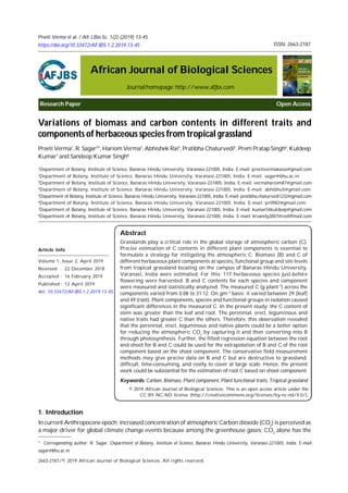
4. Results
4.1. Species Composition
A total of 117 herbaceous species belonging to 95 genera and 31 families were recorded from the campus of
Banaras Hindu University. The family Poaceae had the highest species number (19) and fifteen families had
single species. Amongall the families, the four families (Poaceae, Asteraceae, Fabaceae, and Cyperaceae) were
species-rich (Appendix 1). On the basis of dry B (g plant-1
); Aurobindo donex, Anisomelos indica and Hyptis
suveolens were dominant species in the study area (Appendix 1).
4.2. B and C Across the Species and Components
The statistical analysis implied that the plant B
and C differed significantly due to species
(F116,1170 = 61, P  0.0001 and F116,1170 = 61,
P  0.0001), plant components (F2,1170 = 248, P
 0.0001 and F2,1170 = 279, P  0.0001) and their
interactions(F232, 1170= 11, P  0.0001and F232,
1170 = 12, P  0.0001).
Across the species and components;
maximumB (gplant-1
)forleaf(46.04),stem(65.49),
and shoot (11.53) components as well as for total
plant (133.85) were represented by A. donex,
whilemaximumrootB wasexhibited byRauwolfia
serpentina(25.58). Conversely; theminimum B for
leaf (0.19), stem (0.08) and shoot (0.16)
components were showed by Polygonum
barbatum, Lippia alba, Tanacetum parthenium,
respectively. Further, Lindernia anagallis had
minimum root (0.01) as well as total plant (0.37)
B (Appendix 1). Interestingly, these species also
exhibited similar patterns regarding the
maximum and minimumvalues for C content on
g plant-1
basis. For instance; the observed C for
leaf, stem, shoot, root and total plant varied from
0.08 (P. barbatum) to 20.20 (A. donex), 0.03 (L. alba)
to 31.12 (A. donex), 0.07 (T. parthenium) to 51.31
(A. donex), 0.004 (L. anagallis) to 10.88
(R. serpentina) and 0.15 (L. anagallis) to 60.69 (A.
donex), respectively (Appendix 1).
Species-wise, the measured C from dry B for
leaf, stem, shoot, root and total plant ranged
between 37 (Rorippa dubia) and 47 (Phyllanthus
asperalatus), 38 (L. anagallis and L. alba) and 48
(Cassia tora, Cleome viscosa, Croton bonplandianus,
Desmodium gangeticum, Desmostachya bipinnata,
Hyptis suveolens, Melilotus indica, P. asperalatus,
Rauvolfia serpentine, Saccharum munja, S.
spontaneum, Scoparia dulcis, Sida rhomboidea and
Vetiveria zizanoidies), 38 (Trianthema
portulacastrum) and 47 (C. viscosa, C.
bonplandianus), 36 (H. suveolens) and 50 (Digitaria
ciliaris), and 39 (R. dubia) and 47 (C.
bonplandianus), respectively.
The average B partitioning into the different
plant components indicated that the shoots had
Figure 1: Mean biomass (g plant-1
), carbon content (g plant-1
)
and carbon to biomass ratio based on 117 herbaceous species
for different plant components in the tropical grassland at
Varanasi, India. Bars affixed with different letters within each
component are significantly different from each other.
Meanbiomass(gPlant-1)
0
4
8
12
16
Meancarbon(gPlant
-1
)
0
2
4
6
8
Plant components
Leaf Stem Shoot Root Total
Meancarbontobiomassratio
0.0
0.2
0.4
0.6
a
b
c
d
e
a
b
c
d
e
0.43
a
0.45
a
0.44
a
0.41
a
0.43
a

five times greater B than theroots (Figure 1). More or lesssimilar trend was also exhibited byC portioning into
different plant components (Figure 1). Thepatterns ofB, as well as Cacross the plant components,significantly
varied in the order of stem>leaf>root as suggested by the Tukey’s HSD analysis (Figure 1).
4.3. Functional Group Effects on B and C
ANOVA showed that B and C contents of different plant components differed substantially due to variations
in the functional groups related to nativity and growth forms (Table 1). The plant components of life form
functional groupsalso changed notably dueto variationsintheir B and Ccontents, except B aswellas C of root
component and whole plant B. For lifespan functionalgroup; only B and C of root component as well as whole
plant varied statistically (Table 1).
Variables
Species Family Lifespan Nativity Lifeform Growth form
F116,390
F30,476
F2,504
F2,504
F3,503
F3,503
Leaf biomass 30.82*** 4.20* 2.49ns
10.14*** 3.12* 4.46**
Leaf carbon 31.50*** 3.92* 2.55ns
10.24*** 3.43* 4.39*
Stem biomass 29.71*** 5.94** 1.94ns
7.12** 3.31* 6.13**
Stem carbon 30.07*** 5.98** 2.07ns
7.02** 3.36* 6.27**
Shoot biomass 33.80*** 5.38** 2.28 ns 8.60*** 2.89* 5.67**
Shoot carbon 33.66*** 5.29** 2.38 ns 8.50*** 3.09* 5.75**
Root biomass 13.79*** 4.24* 8.41*** 18.64*** 0.56ns
2.92*
Root carbon 13.61*** 4.12* 8.39*** 18.86*** 0.62ns
2.91*
Total biomass 33.98*** 5.38** 3.49* 10.61*** 2.51ns
5.49**
Total carbon 33.70*** 5.28** 3.50* 10.40*** 2.72* 5.61**
Root:shoot carbon ratio 9.98*** 11.40*** 10.37*** 7.91*** 0.81ns
17.28***
Table 1: Summary of ANOVA (F-value and degree of freedom) of dry weight (biomass) and carbon contents
in different plant components of herbaceous species due to variations in species, family, lifespan, nativity, life
and growth forms.
Note: The one, two and three asterisks superscripted on different F-values indicate the significance levels at *P  0.01,
**P  0.001, ***P  0.0001 and ns
insignificant. The subscripted values to the F indicated the degree of freedom.
Results showed that the perennials, native, grasses and erect functional group categories represented
greater B and C in their stems compared to other components of the functional groups (Table 2). Their
corresponding S: R ratios for B and C ranged from 4.3 to 4.7, 4.2 to 4.5, 5.3 to 5.8, and 5.4 to 5.9. Annual, non-
native, legume and decumbent functional group categories had 6.8 and 7.5, 6.5 and 7.2, 5.5 and 6.3, and 6.4
and 6.9 times higher shoot B and C than their root components. Interestingly; perennial, cosmopolitan, sedge,
and prostate functionalgroups represented the lowest shoot to root (highest root toshoot) ratios for B and C in
their respective functional groups (Table 2).
4.4. Effects of site on B and C contents (g m-2
)
Statistical analysis showed that the sites caused significant difference in the herbaceous species (F2, 42: 33.06,
P  0.001) which varied from 9 (site-3) - 15 (site-2). Analysis further revealed that sites substantially influenced
the B and C contents of leaf (F2, 42: 9.31, P  0.001 and F2, 42: 8.92, P  0.001), shoot (F2, 42: 10.56, P  0.001 and
F2, 42: 10.64, P  0.001), root components (F2, 42: 13.96, P  0.001 and F2, 42: 13.50, P  0.001) and whole plant
(F2, 42: 25.09, P  0.001 and F2, 42: 23.90, P  0.001). For example, across the sites; the B and C contents of leaf,
stem, shoot, root components, and whole plant ranged from 48 to 102 and 21 to 42, 70 to 94 and 31 to 42, 118
to 195 and 51 to 85, 73 to 184 and 29 to 75, and 192 to 380 and 81 to 160, respectively (Table 3). The trend
showed that the values of these variables for different plant components were lowest at highly disturbed
location (site-3) and highest at less disturbed (site-1) location (Table 3).

Table 2: Mean herbaceous biomass; B (g plant-1
), carbon; C (g plant-1
), C to B ratios and for different plant trait
categories in tropical grassland. Values in parentheses are ± 1SE.
Plant components Annual Biennial Perennial
Leaf biomass (B) 4.50 (0.66) 4.90 (0.98) 5.63 (1.13)
Leaf Carbon (C) 1.94 (0.29) 2.01 (0.40) 2.43 (0.49)
C:B ratio 0.431 0.411 0.432
Stem biomass 4.95 (1.22) 6.17 (2.26) 7.06 (1.76)
Stem carbon 2.27 (0.58) 2.77 (1.01) 3.31 (0.83)
C:B ratio 0.459 0.451 0.467
Shoot biomass 9.45 (1.81) 11.07 (3.15) 12.69 (2.84)
Shoot carbon 4.22 (0.84) 4.78 (1.37) 5.75 (1.31)
C:B ratio 0.447 0.436 0.452
Root biomass 1.38 (0.56) 1.84 (0.43) 2.96 (0.69)
Root carbon 0.56 (0.10) 0.74 (0.17) 1.22 (0.29)
C:B ratio 0.404 0.403 0.410
Total biomass 10.83 (2.02) 12.91 (3.33) 15.65 (3.34)
Total C 4.78 (0.93) 5.52 (1.45) 6.97 (1.51)
C:B ratio 0.442 0.426 0.444
Native Non-native Cosmopolitan
Leaf biomass 7.77 (1.99) 4.22 (0.50) 4.06 (2.21)
Leaf carbon 3.36 (0.87) 1.82 (0.22) 1.73 (0.96)
C:B ratio 0.432 0.432 0.427
Stem biomass 9.80 (3.16) 4.92 (0.91) 2.45 (1.19)
Stem carbon 4.56 (1.49) 2.27 (0.43) 1.11 (0.52)
C:B ratio 0.464 0.462 0.452
Shoot biomass 17.56 (5.09) 9.14 (1.35) 6.51 (2.28)
Shoot carbon 7.93 (2.33) 4.09 (0.63) 2.84 (0.98)
C:B ratio 0.452 0.458 0.438
Root biomass 4.21 (1.27) 1.41 (0.18) 4.07 (1.99)
Root carbon 1.75 (0.54) 0.57 (0.07) 1.68 (0.84)
C:B ratio 0.416 0.405 0.411
Total biomass 21.77 (6.05) 10.54 (1.48) 10.57
Total carbon 9.68 (2.73) 4.66 (0.68) 4.51
C:B ratio 0.445 0.443 0.432

Table 2 (Cont.)
Forbs Grasses Legumes Sedges
Leaf biomass 4.56 (0.60) 7.77 (2.55) 4.61 (1.85) 3.91 (0.70)
Leaf carbon 1.94 (0.26) 3.42 (1.13) 2.07 (0.84) 1.64 (0.30)
C:B ratio 0.424 0.439 0.451 0.421
Stem biomass 5.87 (1.14) 8.69 (3.72) 5.94 (2.77) 1.20 (0.20)
Stem carbon 2.70 (0.54) 4.12 (1.77) 2.81 (1.32) 0.53 (0.09)
C:B ratio 0.457 0.473 0.462 0.446
Shoot biomass 10.43 (1.69) 16.46 (6.17) 10.55 (4.60) 5.11 (0.83)
Shoot carbon 4.64 (0.77) 7.54 (2.86) 4.88 (2.15) 2.17 (0.36)
C:B ratio 0.445 0.454 0.461 0.426
Root biomass 1.95 (0.39) 3.10 (1.25) 1.91 (0.91) 1.80 (0.40)
Root carbon 0.80 (0.17) 1.29 (0.53) 0.78 (0.37) 0.72 (0.16)
C:B ratio 0.412 0.414 0.409 0.410
Total biomass 12.38 (1.93) 19.56 (7.26) 12.46 (5.43) 6.91 (1.21)
Total carbon 5.44 (0.87) 8.82 (3.31) 5.65 (2.49) 2.89 (0.51)
C:B ratio 0.441 0.451 0.454 0.421
Erect Prostate Procumbent Decumbent
Leaf biomass 5.67 (0.78) 3.83 (1.12) 2.10 (1.15) 3.08 (1.07)
Leaf carbon 2.45 (0.34) 1.65 (0.49) 0.87 (0.48) 1.32 (0.47)
C:B ratio 0.431 0.432 0.415 0.429
Stem biomass 7.34 (1.34) 2.42 (0.55) 2.09 (1.22) 2.39 (1.06)
Stem carbon 3.43 (0.64) 1.08 (0.25) 0.88 (0.49) 1.04 (0.46)
C:B ratio 0.466 0.451 0.424 0.440
Shoot biomass 13.01 (2.08) 6.24 (1.61) 4.19 (2.36) 5.47 (2.06)
Shoot carbon 5.87 (0.96) 2.73 (0.71) 1.75 (0.96) 2.36 (0.90)
C:B ratio 0.450 0.438 0.423 0.432
Root biomass 2.39 (0.45) 1.82 (0.46) 0.83 (0.63) 0.86 (0.26)
Root carbon 0.99 (0.19) 0.74 (0.19) 0.33 (0.24) 0.34 (0.10)
C:B ratio 0.413 0.412 0.401 0.400
Total biomass 15.41 (2.42) 8.07 (1.74) 5.02 (2.99) 6.33 (2.20)
Total carbon 6.86 (1.10) 3.47 (0.76) 2.08 (1.20) 2.70 (0.96)
C:B ratio 0.444 0.432 0.413 0.425

Vegetation parameters Less (Site-1) Medium (Site-2) High (Site-3)
Leaf biomass 101.56 59.80 48.80
(13.18) (7.72) (4.05)
Leaf carbon 42.45 25.06 20.61
(5.55) (3.30) (1.76)
Stem biomass 93.86 85.47 69.51
(10.20) (10.58) (5.56)
Stem carbon 42.29 38.09 30.99
(4.58) (4.72) (2.51)
Shoot biomass 195.42 145.27 118.31
(16.06) (10.85) (7.70)
Shoot carbon 84.77 62.82 51.35
(6.96) (4.68) (3.40)
Root biomass 184.49 109.66 73.45
(23.73) (9.71) (5.63)
Root carbon 74.87 43.00 29.12
(10.07) (3.93) (2.31)
Total biomass 379.91 254.92 191.76
(28.59) (13.11) (10.33)
Total carbon 160.46 106.16 80.75
(12.65) (5.35) (4.42)
Table 3: Mean value of herbaceous biomass (g m-2
) and carbon content (g m-2
) of herbaceous species at three
locations of tropical grassland differing in disturbance intensity. Values in parentheses are ± 1SE.
The mean C: B ratios for different plant components varied between 0.41 (root) and 0.45 (stem). Root had
comparatively larger variability (0.36 to 0.50) than the other traits, while the whole plant expressed least (0.39-
0.47) variability in the C: B ratios (Table 4). Thus, the results suggested that the C predictionbased on C: B ratio
for the whole plant will be more consistent.
Ratios Range Mean
Root to shoot biomass 0.02-9.88 0.41 (0.106)
Root to shoot carbon 0.02-10.50 0.40 ( 0.110)
Carbon to biomass ratio for Leaf 0.37-0.47 0.43 (0.002)
Carbon to biomass ratio for Stem 0.38-0.48 0.45 (0.002)
Carbon to biomass ratio for Root 0.36-0.50 0.41 (0.002)
Carbon to biomass ratio for Shoot 0.38-0.47 0.44 (0.002)
Carbon to biomass ratio for total plant 0.39-0.47 0.43 (0.002)
Table 4: Variations in different ratios related to carbon and biomass of different herbaceous plant components
across the species in a tropical grassland at Varanasi, India. Values in the parentheses are ±1SE.
4.5. Relationships Between Root and Shoot Components Related to B and C Contents
Various significant regression equations betweenshoot (X) and root (Y) based on B and C contents considering
species as data points are shown in Figure 2. Among these significant equations; the considerable R2
(determinationcoefficient) varied from0.27(logarithmic equation for C content) to 0.52 (power equation for B).

Shoot biomass (g plant-1)
0 20 40 60 80 100 120
Rootbiomass(gplant-1)
0
5
10
15
20
25
30
Linear
Logarithmic
Power
Exponential
RB = 0.56 + 0.15SB, R
2
= 0.46, SEE = 2.72, P = 0.0001
RB = -0.22 + 1.48 lnSB, R
2
= 0.28, SEE = 3.15, P = 0.0001
RB = 0.27(SB)0.76, R2 = 0.52, SEE = 2.56, P = 0.0001
RB = 0.55 e
0.05SB
, R
2
= 0.33, SEE = 2.81, P = 0.0001
Shoot carbon (g plant-1)
0 10 20 30 40 50 60
RootCarbon(gplant-1)
0
2
4
6
8
10
12
Linear
Logarithmic
Power
Exponential
RC = 0.24 + 0.13SC, R
2
= 0.45, SEE = 1.15, P = 0.0001
RC = 0.42 + 0.61 lnSC, R2 = 0.27, SEE = 1.33, P = 0.0001
RC = 0.21(SC)
0.75
, R
2
= 0.51, SEE = 1.12, P = 0.0001
RC = 0.62 e
0.05SC
, R
2
= 0.42, SEE = 1.19, P = 0.0001
(a)
(b)
Similarly, theStandard Error ofEstimate(SEE) ranged between1.12(power equationfor C)and 3.15(logarithmic
equation for B). In both the cases; next, to the power equation, the maximum R2 (0.46; for B, and 0.45; for C
content) and minimum SEE (2.72; for C content and 1.15; for B) was exhibited bythe linear equation(Figure 2).
Figure 2: Linear and non-linear relationships (a) between shoot biomass; SB (X-axis) and root biomass;
RB (Y-axis), and (b) between shoot carbon; SC (X-axis) and root carbon; RC (Y-axis) based on 117 herbaceous
species in the tropical grassland at Varanasi, India. R2
=Determination coefficient, SEE = Standard Error of
Estimate, P = level of significance.

5. Discussion
5.1. Species-wise B and C contents
A. donax showed maximum above ground B and C contents; hence, this could be used as an energy crop. It is
advocated because of the greater photosynthetic capacity of A. donax in full sunlight compared to other C3
plants as suggested by Webster et al. (2016). The B production of A. donax in terms of energy and at the same
time reduction of atmospheric CO2
seems to be an interesting observation (Lewandowski et al., 2003). Further,
reports indicated that A. donax may reach B yields up to 100 t ha-1
in the second or third year of cultivation
under the suitable climate and irrigation (Vasconcelos et al., 2007). It forms dense stands on highly disturbed
lands (Saltonstall and Bonnett, 2012), highly fire-tolerant species and having a high level of carbohydrates in
its cell walls (67.85 % dry weight; Scordia et al., 2010; and Chandel et al., 2011), hence, could be a valuable
species for C sequestration and a suitable substrate for ethanol production (Scordia et al., 2010; and Chandel
et al., 2011).
The average total C of herbaceous species was 42.72% of their dry biomass. Similar to the present study,
Davies et al. (2011) also reported 42.02% C of the dry biomass for the herbaceous species. Tumuluru (2015)
reported 43.92 and 42.08% C of the dry biomass for the corn stover and switchgrass, respectively. However, in
various studies, it was around 45% of the plant dry biomass (Olson et al., 1983; and Wang et al., 1999). Across
the species, percent of total above-ground C on the dry-weight basis from steppe grassland of Inner Mongolia,
China has been reported in a range of 15 to 41 having 29 as mean value (Sagar et al., 2017). The percent below
ground C on the dry weight basis was 40.60. The NGGI Workbook 4.2 Revision 2 (1997) assumed 42% C of the
root dry matter for crops and grasses.
The study showed 51 – 85 (gm-2
) above ground C. Based on 0.43 C: B ratio, other studies also reported 44 to
154 (gm-2
) above ground C in an N-input study from the study area (Verma et al., 2013 and 2015). In a steppe
grassland of Inner Mongolia, China it was in a range of 7.12 to 10.72 (Sagar et al., 2017) while in other studies
of USA, the value was around 140-150 (Golubiewski, 2006; and Davies et al., 2011). Thus, the above ground C
in the present study fall under these reported ranges; viz: 7.12 (Sagar et al., 2017) and 150 (Golubiewski, 2006;
and Davies et al., 2011).
5.2. Plant Component-wise C Content
Similar to the present study, significant variations in the root, stem and leaf B and C contents were reported by
Poorter and Bergkotte(1992). The percentage above ground C was substantially higher than the below-ground
C whichsignified the dependencyofthe plant growth onthe supply of Cfrom theshoots, and the nutrientsand
water from the roots. Thus, the assimilation of C by foliage and the acquisition of mineral nutrients and water
by fine roots are balanced with the utilization of C and nutrients in the plants (Cannell and Dewar, 1994).
Further, the C allocation to above ground and below ground plant parts are facilitated by nitrogen supply via
regulatingthe cytokinins and sucrose productions (Vander Werf and Nagel, 1996). Thecytokinins and sucrose
productions through N supply could be other reason for allocating greater C in the stem than the other organs
(Vander Werfand Nagel, 1996). Notably greater C in stem compared to root and leaf could be due to storage of
greater B in stem component than the others because the stem part of the plant has been reported to contain a
comparatively higher concentration of lignin than the leaves and roots (Poorter and Bergkotte, 1992).
5.3. Functional traits-wise C content
In the present study, the perennial plants stored more C and B in comparison to annual and biennial plants
which could be attributable to the excess accumulation of photosynthates in form of carbohydrates, lipids and
other chemical compounds (Dickson, 1989). Since the present study area experienced a marked seasonality,
hence, this storage reserve material could be used by the plants for their respiration and maintenance during
the dormant season (Dickson, 1989). It has been argued that in the seasonal environments, perennial plants
have the ability to fix and store enoughC, over the growingseason to survive the winter and emergefollowing
the year (Farrar et al., 2014) and different speciesincorporatesdifferent C according to their specific metabolism
(Liu et al., 2017).
Among all life form categories, the legumes had relatively more C compared to others. It may be further
linked to their nitrogen-fixing ability in their root nodules which is utilized by such plants for their B and C
production.Probably, itcould bea reasonforconsideringthe leguminousplant asakeydriver forCsequestration
in many studies (Fornara and Tilman, 2008; and Wu et al., 2016). On the other hand, grasses showed high B
(84.2 %) and C allocation above ground compared to the below ground (15.8%). Similar to our results,

Irving (2015) also reported 80-85 % B in above ground and only 15 -20% in below-ground components of the
grasses.
The study suggested that erect plant trait harbored greater B and C than the other traitswhich could be due
to the availabilityofsufficient light to capture the atmospheric C. It is well-known fact that light is animportant
limiting factor for the growth and B build-up in the plants (Neufeld and Young, 2003). As observed in other
studies; the tall plants were thought to be more competent in atmospheric C capturing and B build-up and
outshade the short-statured species (Diekmann and Falkengren-Grerup, 2002). Thus, the erect plant species
had greater B and C than the prostrate and short-statured plants due to their high C capturing ability in
presence of sufficient sunlight (Sagar et al., 2012; and Verma et al., 2015). Greater uptake of atmospheric CO2
into the B of erect trait through the photosynthesis (Cardinale et al., 2012), benefits the storage of CO2
into the
soil as soil organic-C (Fornara and Tilman, 2008; Cong et al., 2014; and Sagar et al., 2017), hence, such trait
could be a strategy in sequestering the C into the soil as organic-C against the problem of global warming.
The notable changes in above ground and below ground C partitioning (R:S ratio) based on C content due
to differences in species, lifespan, nativity and growth forms could be related to the deeper and denser rooting
systems. The deeper, larger and denser rooting systems accumulate greater B and C in below ground than the
above ground and aremore beneficial for the accumulationof C into the soil (Rasmussen et al., 2010). Inpresent
study; R. serpentine, Evolvulus alsinoidis, Convolvulus prostatus, Boerhavia diffusa, Alysicarpus vaginalis, Lauania
procumbence, Ruellia tuberosa and Vetiveria zizanoidies have high R:S ratio because of deeper and denser rooting
systems that could have facilitated greater resource allocation in the roots (Coleman and McConnaughay,
1995; and Poorter et al., 2012).
5.4. Impact of disturbances on B and C
Studies have suggested that grazers increase soilcompaction, disturb soil aggregates and decrease thestability
of soil aggregate, and change thesoil structure. Compact soils showlower porosity, higher bulk density; lower
moisture content due to reduced water infiltration and increased run-off/drainage reduced plant available
water and reduced soilaeration. Further, biotic disturbances reducesoil organic matter, depleteclay content in
the soil and reduce soil structure, increase soil erosion and reduction of topsoil, generating the denser subsoil
exposed, promoting higher bulk density at the soil surface (See Sagar and Verma for greater detail) and
ultimately, loss of herbaceous B and C. Moreover, reduction in B and C along the disturbance gradient may be
argued because of harvesting of above-ground herbage cover which may inhibit the oxygen level in theroots,
consequently, there could be a failure of reproduction and death of a certain individual (Matayaya et al., 2017).
The above ground herbaceous plant component is related to the photosynthetic tissue of the plant. Hence, the
removal of the above-ground herbage cover results in the reduction of the plants’ photosynthetic tissue which
causes loss of carbon and nutrients for growth and development of the plants (Ferraro and Oesterheld, 2002)
and reduction in the herbaceous biomass (Leriche et al., 2003). Therefore, biotic pressure modulated these
conditions and synergistically reduced the B and C contents of the herbaceous species.
5.5. C:B as a C estimator
In prediction analysis for selecting a suitable model, it is necessary to test all reasonable models as rigorously
as possible against known standards to avoid summary judgment based on a single data set (Colwell and
Coddington, 1994) becausethe utility of a model generally depends on its ability topredict unknownvalue for
a given known value (Systat, 2009). Further, higher correlation coefficient, lower standard error of estimate
(standard error of estimate quantifies the spread of the real data points around the fitted regression curve),
least discrepancy in prediction (Sagar et al., 2003; and Systat, 2009) and wide adaptability with minimum time
and cost epitomize the performance and utility the of model (Colwell and Coddington, 1994; and Xie et al.
2009). For estimation of root C using different regression equation (based on root and shoot C), the power
equation had higher correlation coefficient and lowest SEE than the others, thus, C: B ratio could be an
appropriate estimator of the C content.
6. Conclusion
Comparatively greater C in perennials, erects, legumes and native trait categories than the others suggested
that the species having such traits could be used for reducing the atmospheric CO2
by capturing it and then
converting into the B through the photosynthesis. The conservative field measurement methods may give
precise data onB and C, but are destructive to grassland, difficult, time-consuming, and costly tocover at large

scale, hence, the C:B ratio could be used as an estimator of C at species, components, functional group and site
levels in the tropical grassland.
Acknowledgment
R. Sagar is thankful to the SERB, New Delhi for the financial support with file number: EEQ/2016/000129. PV
is supported by University Grants Commission, New Delhi.
Conflicts of interest
We declare that we have no conflicts of interest.
References
Alley, R.B. (2016). A heated mirror for future climate. Science, 352 (6282), 151-152.
Barbosa, R.I., dos Santos, J.R., da Cunha, M.S., Pimentel, T.P. and Fearnside, P.M. (2012). Root biomass, root:
shoot ratio and belowground carbon stocks in the open savannahs of Roraima, Brazilian Amazonia. Aust.
J. Bot., 60, 405-16.
Blanc, L., Echard, M., Herault, B., Bonal, D., Marcon, E., Chave, J. and Baraloto, C. (2009). Dynamics of
aboveground carbon stocks in a selectively logged tropical forest. Ecol. Appl., 19, 1397-1404.
Bolinder, M.A., Angers, D.A., Be´langer, G., Michaud, R., and Laverdie‘re, M.R. (2002).Root biomass and shoot
to root ratios of perennial forage crops in eastern. Canada Can. J. Plant Sci., 82, 731-737.
Broecker, W.S. (1975). Climate change: are we on the brink of a pronounced global warming? Science, 189,
460–463.
Bunker, D.E., de-Clerck, F., Bradford, J.C., Colwell, R.K., Perfecto, I., Phillips, O.L., Sankaran,M. and Naeem, S.
(2005). Species loss and above-ground carbon storage in a tropical forest. Science, 310, 1029–1031.
Cannell, M.G.R. and Dewar, R.C. (1994). Carbon allocation in trees: a review of concepts for modelling. In:
Begon, M., and Fitter, A. H., eds. Adv Ecol Res., 25, 59–104.
Cardinale, B.J., Duffy, J.E., Gonzalez, A., Hooper, D.U., Perrings, C., Venail, P., Narwani, A., Mace, G.M.,
Tilman, D., Wardle, D.A. and Kinzig, A.P. (2012).Biodiversity loss and its impact on humanity. Nature, 486,
59.
Chandel, A.K., Singh, O.V., Chandrasekhar, G., Rao, L.V. and Narasu, M.L. (2011). Bioconversion of novel
substrate, Saccharum spontaneum, a weedy material into ethanol by Pichia stipitis NCIM3498. Bioresour
Technol., 102, 1709–1714.
Coleman, J.S. and McConnaughay, K.D.M. (1995). A nonfunctional interpretation of a classical
optimalpartitioning example. Funct Ecol., 9, 951–954.
Colwell, R.K. and Coddington, J.A. (1994).Estimating terrestrialbiodiversity through extrapolation. Phil Trans
R Soc Lond, B 345, 101-18.
Cong, W.F., Ruijven, J., Mommer, L., DeDeyn, G.B., Berendse, F. and Hoffland, E. (2014).Plant species richness
promotes soil carbon and nitrogen stocks in grasslands without legumes. J of Ecol., 102, 1163-70.
Davies, Z.G., Edmondson, J.L., Heinemeyer, A.,Leake,J.R. and Gaston, K.J. (2011).Mappinganurbanecosystem
service: quantifying aboveground carbon storage at a citywide scale. J Appl Ecol., 48, 1125-34
De Deyn, G.B., Cornelissen, J.H. and Bardgett, R. D. (2008).Plant functional traitsand soil carbon sequestration
in contrasting biomes. Ecol Lett., 11, 516-31.
Dickson, R. E. (1989). Carbon and nitrogen allocation in trees. Ann Sci Forest, 46, 631s-647s.
Diekmann, M. and Falkengren-Grerup, U. (2002). Prediction of species response to atmospheric nitrogen
deposition by means of ecological measures and life history traits. J of Ecol., 90,108–120. DOI: 10.1046/
j.0022-0477.2001.00639.x
Dinakaran, J., Hanief, M., Meena, A. and Rao, K. S. (2014). The chronological advancement of soil organic
carbon sequestration research: a review. P Natl A Sci India B Journal, 84(3), 487-504.
Duthie, J.F. (1903). Flora of the upper Gangetic plain, and of the adjacent Siwalik and sub-Himalayan tracts.
Office of the Superintendent of Government Printing, Calcutta, India. DOI: 10.5962/bhl.title.21629

Farrar, K., Bryant, D. andCopeSelby, N. (2014). Understanding and engineering beneficial plant–microbe
interactions: plant growth promotion in energy crops. Plant Biotechnol J., 12:1193-206.
Ferraro, D.O. and Oesterheld, M. (2002). Effect of defoliation on grass growth. Quantitat. Rev. Oikos. 98, 125-
133.
Fisher, M.J., Rao, I.M., Ayarza, M.A., Lascano, C.E., Sanz, J.I., Thomas, R.J. and Vera, R.R. (1994). Carbon
storage by introduced deep-rooted grasses in the South-American Savannas. Nature, 371, 236-238.
Fornara, D.A. and Tilman, D. (2008). Plant functional composition influences rates of soil carbon and nitrogen
accumulation. J Ecol., 96, 314–322.
Frank, A.B., Berdahl, J.D., Hanson, J.D., Liebig, M.A. and Johnson, H.A. (2004).Biomassand CarbonPartitioning
in Switchgrass. Crop Sci. 44, 1391-1396.
Gilliam, F.S. (2007). The ecological signicance of the herbaceous layer in forest ecosystems. BioScience, 57, 845–
858.
Golubiewski, N.E. (2006). Urbanization increases grassland carbon pools: effects of landscaping in Colorado’s
Front Range. Ecol Appl., 16, 555–571.
Grace, J.B., San Jose´, J., Meir, P., Miranda, H.S. and Montes, R. A. (2006). Productivity and carbon fluxes of
tropical savannas. J Biogeogr., 33, 387–400.
Hall, D.O. and Scurlock, J.M.O. (1991). Climate change and productivity of natural grasslands. Annals of
Botany, 67, 49-55.
IPCC(2003). Good Practice Guidancefor Land Use, Land UseChange, and Forestry. In: J. Penman, M. Gytarsky,
T. Hiraishi, T. Krug, D. Kruger, R. Pipatti, L. Buendia, K. Miwa, T. Ngara, K. Tanabe and F. Wagner (eds).
National Greenhouse Gas Inventories Programme. IGES, Japan.
IPCC (Intergovernmental Panel on Climate Change) (2014). 5th assessment reports; Impacts, Adaptation and
Vulnerability.
Irving, L.J. (2015). Carbon assimilation, biomass partitioning and productivity in grasses. Agriculture, 5, 1116-
34.
Lal, R. (2010). Beyond Copenhagen: Mitigation climate change and achieving food security through soil
carbon sequestration. Food Security. 2, 169-177
LeQuéré, C., Andres, R.J., Boden, T., Conway, T., Houghton, R.A., House, J.I., Marland, G., Peters,G.P., Vander
Werf, G., Ahlström, A. and Andrew, R.M. (2012). The global carbon budget 1959–2011. Earth Syst Sci Data
Discuss, 5, 1107-1157.
Leriche, H., Le Roux, X., Desnoyers, F., Benest, N. and Simiani, G. (2003). Grass response to clipping in an
African Savanna: testing the grazing optimization hypothesis. Ecol Appl. 13,1346–1354.
Lewandowski, I., Scurlock, J.M., Lindvall, E. and Christou, M. (2003). The development and current status of
perennial rhizomatous grasses as energy crops in the US and Europe. Biomass Bioenergy. 25, 335-61.
Lewis, S.L., Lopez-Gonzalez, G., Sonke, B., Affum-Baffoe, K., Baker, T.R., Ojo, L.O., Phillips, O.L., Reitsma, J.M.,
White, L., Comiskey, J.A. and Ewango, C.E. (2009). Increasing carbon storage in intact African tropical
forests. Nature, 457, 1003–1006.
Lieth, H. (1978). Patterns of primary production in the biosphere. Dowden, Hutchinson & Ross.
Liu, J., Bowman, K.W., Schimel, D.S., Parazoo, N.C., Jiang, Z., Lee, M., Bloom, A.A., Wunch, D., Frankenberg, C.,
Sun, Y. and O’dell, C.W. (2017). Contrasting carbon cycle responses of the tropical continents to the 2015–
2016 El Niño. Science. 358 (6360): http://science.sciencemag.org/content/suppl/2017/10/12/
358.6360.eaam5690.DC1
Lu, X., Kicklighter, D.W, Melillo, J. M, Reilly, J.M. and Xu, L. (2015). Land carbon sequestration within the
conterminous United State: Regional-and-state-level analyses. J Geophys Res-Biogeo. 120, 379-398.
Matayaya, G., Wuta, M. and Nyamadzawoa, G. (2017). Effects of different disturbance regimes on grass and
herbaceous plant diversity and biomass in Zimbabwean dambo systems. International Journal of Biodiversity
Science, Ecosystem Services and management. 13, 181–190.
Mcbrayer, J.F. and Cromack, J.K. (1980). Effect of snowpack on oak-litter breakdown and nutrient release in a
Minnesota forest. Pedobiologia., 20, 47–54.

Minami, K., Goudriaan, J., Lantinga, E.A. and Kimura, T. (1993). Significance of grasslands in emission and
absorptionof greenhouse grasses. In: M.J. Barker (ed). Grasslands for Our World. Wellington, NewZealand:
SIR Publishing.
Mokany, K., Raison, R.J. and Prokushkin, A.S. (2006). Critical analysis of root: shoot ratiosin terrestrialbiomes.
Global Change Biol., 12, 84-96.
Neufeld, H.S. and Young, D.R. (2003). Ecophysiology of the herbaceous layer in temperate deciduous forests.
In: Gilliam, F.S. and Roberts, M.R. (eds), The herbaceous layer in forests of eastern North America. Oxford
University Press, New York, 38–90.
NGGI. (1997).Land UseChange and Forestry. Workbook for Carbon Dioxide fromtheBiosphere.Workbook4.2.
National Greenhouse Gas Inventory Committee 59.
Odiwe, A.I., Olanrewaju, G.O. and Raimi, I.O. (2016). Carbon Sequestration in Selected Grass Species in a
Tropical Lowland Rainforest at Obafemi Awolowo University, Ile-Ife, Nigeria. J Trop Biol Conserv., 13.
Olson, J.S., Watts, J.A. and Allison, L.J. (1983). Carbon in live vegetation of major world ecosystem. Oak Ridge
National Laboratory. Oak Ridge, 50–51.
Pan, Y.D., Birdsey, R.A., Phillips, O.L. and Jackson, R.B. (2013). The structure, distribution, and biomass of the
world’s forests. Annu Rev Ecol Evol Syst, 44,593–622.
Peng, J., Dong, W., Yuan, W., Chou, J., Zhang, Y. and Li, J. (2013).Effectsof increased CO2
on land water balance
from 1850 to 1989. Theor Appl Climatol, 111, 483-95.
Piao, S.L., Fang, J.Y., He, J.S. and Xiao, Y. (2004). Spatial distribution of grassland biomass in China. Acta
Phytoecologica Sinica, 28, 491–498.
Poorter, H. and Bergkotte, M. (1992).Chemicalcomposition of24wild species differingin relativegrowth rate.
Plant Cell Environ., 15, 221–229.
Poorter, H., Niklas, K.J., Reich, P.B., Oleksyn, J., Poot, P. and Mommer, L. (2012). Biomass allocation to leaves,
stems and roots: metaanalyses of interspecific variation and environmental control. New Phytol. 193,30-50.
Rasmussen, J., Eriksen, J., Jensen, E. S., and Jensen, H. H. (2010). Root size fractions of ryegrass and clover
contribute differently to C and N inclusion in SOM. Biol Fertil Soils. 46, 293–297.
Russell, M.B., Domke, G.M., Woodall, C.W. and D’Amato, A. W. (2015).Comparisonsof allometric and climate-
derived estimates of tree coarse root carbon stocks in forests of the United States. Carbon Balance Manag,
10:20.
Sagar, R., Li, G.Y., Singh, J.S. and Wang, S. (2017). Carbon fluxes and species diversity in grazed and fenced
typical steppe grassland of Inner Mongolia, China. J Plant Ecol.
Sagar, R., Pandey, A. and Singh, J.S. (2012). Composition, species diversity, and biomass of the herbaceous
community in dry tropical forest of northern India in relation to soil moisture and light intensity.
Environmentalist, 32, 485–493.
Sagar, R., Raghubanshi, A.S. and Singh, J.S. (2003). Tree species composition, dispersion and diversity along
a disturbance gradient in a dry tropical forest region of India. For Ecol Manage. 186, 61–71.
Sagar, R., Singh, A. and Singh, J.S. (2008). Differential effect of woody plant canopies on species composition
and diversity of ground vegetation: A case study. Trop Ecol., 49, 189–197.
Sainju, U.M., Allen, B.L., Lenssen, A.W. and Ghimire, R.P. (2017). Root biomass, root/shoot ratio, and soil
water content under perennial grasses with different nitrogen rates. Field Crops Res., 210, 183-191.
Sala, O.E. and Paruelo, J.M. (1997). Ecosystem services in grasslands. Nature’s services: Societal dependence on
natural ecosystems. 237-51.
Saltonstall, K. and Bonnett, G.D. (2012). Fire promotes growth and reproduction of Saccharum spontaneum (L.)
in Panama. Biol Invasions, 14,2479–2488.
San Jose, J.J., Montes, R.A. and Farinas, M.R. (1998). Carbon stock and fluxes in a temporal scaling from
savanna to semideciduous forest. For Ecol Manage., 105, 251–262.
Scordia, D., Cosentino, S.L. and Jeffries, T.W. (2010).Second generationbioethanol productionfrom Saccharum
spontaneum L. ssp. aegyptiacum (Willd.), Hack Biores Technol., 101, 5358-5365.

Singh, J.S., Singh, S.P. and Gupta, S.R. (2006). Ecology, Environment and Resource Conservation. Anamaya
Publishers, New Delhi, India.
Singh, V., Singh, H., Sharma, G.P. and Raghubanshi, A.S. (2011).Eco-physiological performance of twoinvasive
weed congeners (Ageratum conyzoides L. and Ageratum houstonianum Mill.) in the Indo-Gangetic plains of
India. Environ Monit Assess, 178,415-422.
SYSTAT. (2009). Systat Software, Inc. San Jose, CA. www.systat.com
Thomas, S.C. and Martin, A.R. (2012). Carbon content of tree tissues: a synthesis. Forests, 3, 332-352.
Tumuluru, J.S. (2015). Comparison of chemical compositionand energy property of torrefied switchgrass and
corn stover. Front Energy Res., 3, 46.
UNFCCC (United Nations Framework Convention on Climate Change). (2015). About the United Nations
framework convention on climate change.
Van der, Werf, A. and Nagel, O.W. (1996). Carbon allocation to shoots and roots in relation to nitrogen supply
is mediated by cytokinins and sucrose: Opinion. Plant Soil., 185, 21-32.
van Soest, P.J. (1963). Use of detergents in the analysis of fibrous feeds. I. preparation of fiber residues of low
nitrogen content. J Assoc off Agr Chem., 46, 825-829.
Vasconcelos, G.C., Gomes, J.C. and Corrêa, L.A. (2007). Rendimento de biomassa da Cana-do-Reino (Arundo
donax L.). Boletim de Pesquisa e Desenvolvimento, 42. Pelotas: Embrapa Clima Temperado.
Verma, D.M., Pant, P.C. and Hanfi, M.I. (1985). Flora of Raipur, Durg and Rajnandgaon. Flora of India. Series
3. Botanical Survey of India, Howrah, India.
Verma, P., Sagar, R., Verma, H., Verma, P. and Singh, D.K. (2015). Changes in species composition, diversity
and biomass of herbaceous plant traits due to N amendment in a dry tropical environment of India. J of
Plant Ecol ., 8, 321-332.
Verma, P., Verma, P. and Sagar, R. (2013).Variationsin N mineralizationand herbaceous species diversitydue
to sites, seasons, and N treatments in a seasonally dry tropical environment of India. For Ecol Manage., 297,
15-26.
Wang, S.Q., Zhou, C.H. and Luo, C.W. (1999). Studying carbon storagespatialdistribution of terrestrialnatural
vegetation in China. Prog Geogr., 18, 238–244.
Webster, R.J., Driever, S.M., Kromdijk, J., McGrath, J., Leakey, A.D., Siebke, K., Demetriades-Shah, T., Bonnage,
S., Peloe, T., Lawson, T. and Long, S.P. (2016). High C3 photosynthetic capacity and high intrinsic water
use efficiency underlies the high productivity of the bioenergy grass Arundo donax. Sci Rep. 6, 20694.
White, R., Murray, S. and Rohweder, M. (2000). Pilot analysis of global ecosystems: Grassland ecosystems.
World Resources Institute, Washington, D.C. 69.
Wu, G.L., Liu, Y., Tian, F.P. and Shi, Z.H. (2016). Legumes functional group promotes soil organic carbon and
nitrogen storage by increasing plant diversity. Land Degrad Dev., 28, 1336-44.
Xie, J., Li, Y., Zhai, C., Li, C. and Lan, Z. (2009). CO2
absorptionby alkaline soils and itsimplication to theglobal
carbon cycle. Environ Geol., 56, 953-61.
Yang,Y.H., Fang,J.Y., Ma, W.H., Guo,D.L. and Mohammat, A. (2010).Large-scalepattern ofbiomasspartitioning
across China’s grasslands. Glob Ecol Biogeogr., 19, 268–277.

Herbaceous Species Family Components Biomass (B) Carbon (C) C:B Discre1
Acalypha indica Euphorbiaceae Shoot 2.65 (0.19) 1.17 (0.08) 0.44 2.61
L.E,A,NLF,N
Root 0.39 (0.03) 0.16 (0.01) 0.41 –4.81
Stem 1.12 (0.15) 0.52 (0.07) 0.46 7.38
Leaf 1.53 (0.18) 0.65 (0.07) 0.42 –1.22
Total 3.03 (0.19) 1.33 (0.08) 0.44 2.04
Achyranthes aspera Amaranthaceae Shoot 28.41 (1.12) 12.36 (0.48) 0.44 1.16
L. E,Bi,NLF,N
Root 1.92 (0.59) 0.79 (0.28) 0.41 –4.51
Stem 19.08 (1.02) 8.46 (0.45) 0.44 3.02
Leaf 9.33 (0.55) 3.90 (0.23) 0.42 –2.87
Total 30.33 (1.41) 13.15 (0.66) 0.43 0.82
Aerva sanguinolenta Amaranthaceae Shoot 3.22 (0.73) 1.45 (0.34) 0.45 4.51
L. E,Pe,NLF,N
Root 0.81 (0.11) 0.35 (0.06) 0.43 0.49
Stem 1.71 (0.43) 0.78 (0.20) 0.46 5.73
Leaf 1.50 (0.30) 0.67 (0.14) 0.45 3.73
Total 4.03 (0.82) 1.79 (0.39) 0.44 3.19
Ageratum conyzoides Asteraceae Shoot 1.55 (0.40) 0.71 (0.18) 0.46 6.13
L. E,A,NLF,NN
Root 0.13 (0.04) 0.05 (0.02) 0.38 –11.80
Stem 0.67 (0.16) 0.31 (0.08) 0.46 7.06
Leaf 0.89 (0.24) 0.40 (0.11) 0.45 4.33
Total 1.68 (0.43) 0.76 (0.20) 0.45 4.95
Ageratum houstonianumAsteraceae Shoot 8.86 (2.79) 3.94 (1.27) 0.44 3.30
L. E,A,NLF,NN
Root 0.95 (0.28) 0.38 (0.11) 0.40 –7.50
Stem 5.37 (1.81) 2.47 (0.85) 0.46 6.51
Leaf 3.49 (1.02) 1.47 (0.44) 0.42 –2.09
Total 9.80 (3.01) 4.32 (1.36) 0.44 2.45
Alternanthera sessilus Amaranthaceae Shoot 9.62 (2.37) 4.21 (1.04) 0.44 1.74
L. P,A,NLF,NN
Root 0.78 (0.14) 0.31 (0.05) 0.40 –8.19
Stem 3.98 (1.01) 1.76 (0.45) 0.44 2.76
Leaf 5.64 (1.40) 2.45 (0.60) 0.43 1.01
Total 10.41 (2.47) 4.51 (1.07) 0.43 0.75
Table A1: Species-wise variation in mean dry biomass (g plant-1
), carbon content (g plant-1
), carbon to biomass
ratio (C: B) and percent discrepancy in prediction based on average C: B (Discre1
= 0.43) herbaceous species
occurred in tropical grassland at Varanasi, India. Values in parentheses are ± 1SE. The abbreviations used; AGB
= above ground dry biomass, RB = root biomass, E = Erect, P = Prostrate, De = Decumbent, Pro = Procumbent, A
= Annual, Bi = Biennial, Pe = Perennial, G = Grasses, Se = sedge, NLF = Non leguminous forbs, LF = leguminous
forbs, N = Native, NN = Nonnative, COS = cosmopolitan.
Appendix

Table A1 (Cont.)
Appendix (Cont.)
Alysicarpus monilifer Fabaceae Shoot 5.14 (0.27) 2.27 (0.11) 0.44 2.63
L.P,Pe,LF,N
Root 1.35 (0.18) 0.53 (0.07) 0.39 –9.53
Stem 2.94 (0.15) 1.33 (0.06) 0.45 4.95
Leaf 2.21 (0.20) 0.94 (0.08) 0.43 –1.10
Total 6.50 (0.35) 2.80 (0.14) 0.43 0.18
Alysicarpus vaginalis Fabaceae Shoot 2.08 (0.13) 0.87 (0.05) 0.42 –2.80
L. De,Pe,LF,N
Root 1.88 (0.16) 0.74 (0.08) 0.39 –9.24
Stem 1.40 (0.08) 0.60 (0.03) 0.43 –0.33
Leaf 0.68 (0.06) 0.27 (0.02) 0.40 –8.30
Total 3.96 (0.17) 1.61 (0.07) 0.41 –5.76
Amaranthus spinosus Amaranthaceae Shoot 17.22 (1.74) 7.04 (0.75) 0.41 –5.18
L. E,A,NLF,NN
Root 5.83 (0.89) 2.35 (0.41) 0.40 –6.68
Stem 8.96 (0.97) 3.64 (0.25) 0.41 –5.85
Leaf 8.25 (2.24) 3.40 (0.91) 0.41 –4.34
Total 23.05 (2.06) 9.39 (0.97) 0.41 –5.55
Amaranthus viridis Amaranthaceae Shoot 2.75 (0.99) 1.12 (0.40) 0.41 –5.58
L.E,A,NLF,NN
Root 0.81 (0.50) 0.30 (0.18) 0.37 –16.10
Stem 1.09 (0.33) 0.44 (0.13) 0.40 –6.52
Leaf 1.66 (0.69) 0.68 (0.28) 0.41 –4.97
Total 3.56 (1.45) 1.42 (0.56) 0.40 –7.80
Ammania baccifera Lythraceae Shoot 1.64 (0.57) 0.72 (0.26) 0.44 2.06
L. E,A,NLF,N
Root 0.12 (0.05) 0.05 (0.02) 0.42 –3.20
Stem 0.79 (0.28) 0.36 (0.13) 0.46 5.64
Leaf 0.85 (0.33) 0.37 (0.15) 0.44 1.22
Total 1.76 (0.58) 0.77 (0.26) 0.44 1.71
Anagallis arvensis Primulaceae Shoot 1.61 (0.88) 0.69 (0.39) 0.43 –0.33
L.E,A,NLF,NN
Root 0.09 (0.03) 0.04 (0.01) 0.44 3.25
Stem 0.48 (0.24) 0.21 (0.11) 0.44 1.71
Leaf 1.13 (0.63) 0.48 (0.28) 0.42 –1.23
Total 1.70 (0.91) 0.73 (0.40) 0.43 –0.14
Anisomalis indica Lamiaceae Shoot 85.47 (6.53) 38.12 (3.34) 0.45 3.59
L. E,Pe,NLF,N
Root 9.78 (3.63) 3.98 (1.39) 0.41 –5.66
Stem 55.97 (6.85) 26.02 (3.16) 0.46 7.51

Table A1 (Cont.)
Appendix (Cont.)
Leaf 29.50 (1.66) 12.10 (0.82) 0.41 –4.83
Total 95.25 (9.37) 42.10 (4.43) 0.44 2.71
Argemon mexicana Papaveraceae Shoot 8.43 (2.70) 3.68 (1.16) 0.44 1.50
L. E,A,NLF,NN
Root 1.13 (0.29) 0.47 (0.13) 0.42 –3.38
Stem 2.46 (0.62) 1.08 (0.26) 0.44 2.06
Leaf 5.97 (2.09) 2.60 (0.91) 0.44 1.27
Total 9.56 (2.97) 4.15 (1.28) 0.43 0.94
Atylosia marmorata Fabaceae Shoot 5.76 (0.30) 2.60 (0.12) 0.45 4.74
Benth.P,A,LF,NN
Root 1.21 (0.24) 0.48 (0.08) 0.40 –8.40
Stem 2.14 (0.24) 0.98 (0.11) 0.46 6.10
Leaf 3.61 (0.19) 1.62 (0.07) 0.45 4.18
Total 6.97 (0.44) 3.08 (0.17) 0.44 2.69
Aurondo donex Poaceae Shoot 111.53 (8.49) 51.31 (4.24) 0.46 6.53
L. E,P,G,NN
Root 22.32 (0.87) 9.37 (0.48) 0.42 –2.43
Stem 65.49 (6.21) 31.12 (2.96) 0.48 9.51
Leaf 46.04 (2.31) 20.20 (1.29) 0.44 1.99
Total 133.85 (8.93) 60.69 (4.51) 0.45 5.16
Blumea lacera Asteraceae Shoot 8.08 (1.51) 3.36 (0.62) 0.42 –3.40
L.E,A,NLF,NN
Root 1.23 (0.26) 0.49 (0.10) 0.40 –7.94
Stem 2.60 (0.69) 1.16 (0.31) 0.45 3.62
Leaf 5.48 (0.85) 2.20 (0.32) 0.40 –7.11
Total 9.31 (1.68) 3.86 (0.69) 0.41 –3.71
Boerhavia diffusa Nyctaginaceae Shoot 7.61 (1.87) 3.28 (0.82) 0.43 0.23
L. Pro,Pe, NLF,Cos
Root 7.42 (3.72) 3.12 (1.67) 0.42 –2.26
Stem 4.81 (1.38) 2.15 (0.62) 0.45 3.80
Leaf 2.79 (0.54) 1.12 (0.22) 0.40 –7.12
Total 15.03 (4.13) 6.39 (1.82) 0.43 –1.14
Caesulia axillaris Asteraceae Shoot 20.87 (0.93) 9.13 (0.29) 0.44 1.71
Roxb. De,A,NLF,N
Root 2.07 (0.32) 0.85 (0.14) 0.41 –4.72
Stem 10.61 (0.65) 4.64 (0.28) 0.44 1.67
Leaf 10.25 (0.52) 4.48 (0.20) 0.44 1.62
Total 22.93 (0.98) 9.98 (0.36) 0.44 1.20

Table A1 (Cont.)
Appendix (Cont.)
Cleome viscosa Capparidaceae Shoot 26.87 (4.91) 12.71 (2.48) 0.47 9.09
L.E,A,NLF,NN
Root 4.10 (1.05) 1.65 (0.34) 0.40 –6.85
Stem 18.91 (3.79) 9.10 (1.84) 0.48 10.65
Leaf 7.96 (1.12) 3.61 (0.65) 0.45 5.19
Total 30.97 (5.70) 14.36 (2.72) 0.46 7.26
Commelina benghalensis Commelinaceae Shoot 13.59 (2.96) 5.58 (1.25) 0.41 –4.73
L. Pro,A,NLF,NN
Root 3.36 (1.00) 1.29 (0.36) 0.38 –12.00
Stem 6.96 (1.67) 2.84 (0.73) 0.41 –5.38
Leaf 6.63 (1.33) 2.75 (0.55) 0.41 –3.67
Total 16.95 (3.59) 6.88 (1.49) 0.41 –5.94
Convolvulus prostratus Convolvulaceae Shoot 2.11 (0.43) 0.87 (0.19) 0.41 –4.29
Forssk. P,Pe,NLF,N
Root 3.66 (0.57) 1.42 (0.23) 0.39 –10.83
Stem 0.84 (0.25) 0.37 (0.11) 0.44 2.38
Leaf 1.26 (0.23) 0.51 (0.11) 0.40 –6.24
Total 5.77 (0.21) 2.30 (0.09) 0.40 –7.87
Coronopus didynamus Brassicaceae Shoot 5.29 (1.36) 2.28 (0.59) 0.43 0.23
L. De,A,NLF,NN
Root 0.29 (0.05) 0.11 (0.02) 0.38 –13.36
Stem 2.57 (0.69) 1.10 (0.30) 0.43 –0.46
Leaf 2.73 (0.67) 1.18 (0.30) 0.43 0.52
Total 5.58 (1.34) 2.39 (0.58) 0.43 –0.39
Croton bonplandianus Euphorbiaceae Shoot 8.76 (1.43) 4.13 (0.68) 0.47 8.79
Baill. E,Pe,NLF,NN
Root 0.83 (0.17) 0.37 (0.09) 0.45 3.54
Stem 7.14 (1.12) 3.40 (0.53) 0.48 9.70
Leaf 1.62 (0.43) 0.73 (0.20) 0.45 4.58
Total 9.58 (1.58) 4.49 (0.75) 0.47 8.25
Cynodon dactylon Poaceae Shoot 2.12 (1.26) 0.97 (0.58) 0.46 6.02
L. P,Pe,G,COS
Root 0.53 (0.14) 0.21 (0.06) 0.40 –8.52
Stem 1.09 (0.70) 0.51 (0.33) 0.47 8.10
Leaf 1.04 (0.56) 0.46 (0.25) 0.44 2.78
Total 2.65 (1.34) 1.18 (0.61) 0.45 3.43
Cyperus brevifolius Cyperaceae Shoot 5.10 (0.32) 2.05 (0.12) 0.40 –6.98
Rottb. E,Pe,Se,NN
Root 1.16 (0.07) 0.46 (0.03) 0.40 –8.43

Table A1 (Cont.)
Appendix (Cont.)
Stem 0.75 (0.10) 0.33 (0.04) 0.44 2.27
Leaf 4.35 (0.23) 1.73 (0.09) 0.40 –8.12
Total 6.26 (0.35) 2.51 (0.13) 0.40 –7.24
Cyperus cyperoides Cyperaceae Shoot 1.93 (0.90) 0.87 (0.41) 0.45 4.61
Kuntze. P,Pe,Se,NN
Root 0.83 (0.18) 0.34 (0.07) 0.41 –4.97
Stem 0.50 (0.17) 0.23 (0.08) 0.46 6.52
Leaf 1.44 (0.73) 0.64 (0.33) 0.44 3.25
Total 2.76 (1.06) 1.22 (0.46) 0.44 2.72
Cyperus difformis Cyperaceae Shoot 7.93 (1.28) 3.19 (0.52) 0.40 –6.89
L. E,A,Se,NN
Root 3.34 (0.17) 1.35 (0.09) 0.40 –6.39
Stem 2.19 (0.40) 0.94 (0.17) 0.43 –0.18
Leaf 5.74 (0.90) 2.25 (0.36) 0.39 –9.70
Total 11.28 (1.38) 4.54 (0.59) 0.40 –6.84
Cyperus esculentus Cyperaceae Shoot 5.89 (0.66) 2.63 (0.31) 0.45 3.70
L. E,M,Pe,Se,N
Root 1.72 (0.49) 0.70 (0.20) 0.41 –5.66
Stem 1.77 (0.26) 0.81 (0.12) 0.46 6.04
Leaf 4.12 (0.44) 1.82 (0.21) 0.44 2.66
Total 7.61 (1.06) 3.33 (0.47) 0.44 1.73
Cyperus iria Cyperaceae Shoot 3.56 (0.45) 1.50 (0.18) 0.42 –2.05
L. E,S,A,Se,NN
Root 1.71 (0.23) 0.69 (0.10) 0.40 –6.57
Stem 0.84 (0.11) 0.38 (0.05) 0.45 4.95
Leaf 2.71 (0.37) 1.12 (0.15) 0.41 –4.04
Total 5.27 (0.58) 2.19 (0.24) 0.42 –3.47
Cyperus killinga Cyperaceae Shoot 3.10 (0.24) 1.25 (0.09) 0.40 –6.64
Endl. E,Pe,Se,NN
Root 1.16 (0.17) 0.46 (0.07) 0.40 –8.43
Stem 0.65 (0.07) 0.27 (0.03) 0.42 –3.52
Leaf 2.45 (0.24) 0.98 (0.09) 0.40 –7.50
Total 4.26 (0.32) 1.71 (0.12) 0.40 –7.12
Cyperus rotundus Cyperaceae Shoot 9.79 (0.47) 4.27 (0.20) 0.44 1.41
L.P,Pe,Se,COS
Root 4.25 (0.43) 1.70 (0.18) 0.40 –7.50
Stem 1.44 (0.10) 0.66 (0.04) 0.46 6.18
Leaf 8.35 (0.38) 3.61 (0.16) 0.43 0.54
Total 14.04 (0.81) 5.97 (0.33) 0.43 –1.13

Table A1 (Cont.)
Appendix (Cont.)
Cyperus strigosus Cyperaceae Shoot 3.54 (0.26) 1.49 (0.11) 0.42 –2.16
L. E,Pe,Se,NN
Root 0.77 (0.06) 0.31 (0.03) 0.40 –6.81
Stem 0.94 (0.08) 0.42 (0.04) 0.45 3.76
Leaf 2.59 (0.20) 1.07 (0.08) 0.41 –4.08
Total 4.31 (0.30) 1.80 (0.12) 0.42 –2.96
Dactyloctenium Poaceae Shoot 8.46 (0.31) 3.58 (0.17) 0.42 –1.61
aegyptium L.De,A,G,NN
Root 0.35 (0.02) 0.14 (0.01) 0.40 –7.50
Stem 2.26 (0.10) 0.99 (0.04) 0.44 1.84
Leaf 6.21 (0.21) 2.59 (0.14) 0.42 –3.10
Total 8.81 (0.32) 3.72 (0.18) 0.42 –1.84
Desmodium Fabaceae Shoot 50.77 (0.19) 23.81 (0.08) 0.47 8.31
gangeticum Root 11.44 (0.13) 4.62 (0.04) 0.40 –6.48
(L.) DC. E,LF,Pe,N
Stem 31.40 (0.42) 14.92 (0.20) 0.48 9.50
Leaf 19.37 (0.43) 8.89 (0.20) 0.46 6.31
Total 62.21 (0.22) 28.43 (0.12) 0.46 5.91
Desmodium trifolium Fabaceae Shoot 1.00 (0.27) 0.47 (0.13) 0.47 8.51
L. E,Pe,LF,NN
Root 0.51 (0.21) 0.20 (0.08) 0.39 –9.65
Stem 0.57 (0.25) 0.27 (0.12) 0.47 9.22
Leaf 0.44 (0.04) 0.20 (0.02) 0.45 5.40
Total 1.51 (0.41) 0.67 (0.17) 0.44 3.09
Desmostachya Poaceae Shoot 35.80 (7.54) 16.75 (3.67) 0.47 8.10
bipinnata (L.) Root 2.23 (0.04) 0.90 (0.02) 0.40 –6.54
Stapf E,Pe,G,NN
Stem 27.94 (6.03) 13.40 (2.82) 0.48 10.34
Leaf 7.85 (1.52) 3.36 (0.87) 0.43 –0.46
Total 38.03 (7.57) 17.66 (3.68) 0.46 7.40
Digitaria ciliaris Poaceae Shoot 1.05 (0.10) 0.47 (0.04) 0.45 3.94
Retz.De,A,G,NN
Root 0.02 (0.01) 0.01 (0.00) 0.50 14.00
Stem 0.52 (0.08) 0.24 (0.04) 0.46 6.83
Leaf 0.52 (0.10) 0.23 (0.04) 0.44 2.78
Total 1.06 (0.10) 0.48 (0.05) 0.46 5.04
Echinochloa colona Poaceae Shoot 4.03 (1.23) 1.85 (0.54) 0.46 6.33
(L.) LinkDe,A,G,NN
Root 1.32 (0.00) 0.51 (0.02) 0.39 –11.29

Table A1 (Cont.)
Appendix (Cont.)
Stem 0.82 (0.15) 0.38 (0.06) 0.46 7.21
Leaf 3.21 (1.08) 1.47 (0.47) 0.46 6.10
Total 5.35 (1.23) 2.36 (0.52) 0.44 2.52
Echinochloa crusgalli Poaceae Shoot 1.91 (0.40) 0.84 (0.18) 0.44 2.23
L. De,A,G,NN
Root 1.31 (0.26) 0.51 (0.09) 0.39 –10.45
Stem 0.55 (0.14) 0.25 (0.06) 0.45 5.40
Leaf 1.36 (0.26) 0.60 (0.12) 0.44 2.53
Total 3.22 (0.64) 1.36 (0.26) 0.42 –1.81
Eclipta alba Asteraceae Shoot 1.54 (0.52) 0.65 (0.23) 0.42 –1.88
L. P,A,NLF,NN
Root 0.21 (0.05) 0.09 (0.02) 0.43 –0.33
Stem 0.67 (0.28) 0.30 (0.13) 0.45 3.97
Leaf 0.88 (0.25) 0.35 (0.10) 0.40 –8.11
Total 1.75 (0.55) 0.74 (0.24) 0.42 –1.69
Eleusine indica Poaceae Shoot 10.78 (0.80) 4.65 (0.26) 0.43 0.31
Gaertn. E,A,G,NN
Root 4.04 (0.66) 1.61 (0.25) 0.40 –7.90
Stem 4.78 (0.97) 1.98 (0.34) 0.41 –3.81
Leaf 6.00 (0.58) 2.67 (0.27) 0.45 3.37
Total 14.82 (0.44) 6.26 (0.15) 0.42 –1.80
Eragrostis tenella Poaceae Shoot 1.20 (0.17) 0.52 (0.07) 0.43 0.77
L. E,Pe,G,NN
Root 0.28 (0.15) 0.11 (0.06) 0.39 –9.45
Stem 0.51 (0.06) 0.24 (0.03) 0.47 8.63
Leaf 0.70 (0.13) 0.29 (0.05) 0.41 –3.79
Total 1.49 (0.32) 0.64 (0.13) 0.43 –0.11
Erigeron bonariensis Asteraceae Shoot 3.61 (1.36) 1.64 (0.61) 0.45 5.35
L.E,A,NLF,NN
Root 0.46 (0.22) 0.18 (0.08) 0.39 –9.89
Stem 1.54 (0.57) 0.73 (0.27) 0.47 9.29
Leaf 2.07 (0.84) 0.91 (0.36) 0.44 2.19
Total 4.07 (1.58) 1.82 (0.69) 0.45 3.84
Euphorbia hirta Euphorbiaceae Shoot 1.91 (0.28) 0.86 (0.12) 0.45 4.50
L. Pro,A,NLF,NN
Root 0.18 (0.03) 0.08 (0.01) 0.44 3.25
Stem 1.16 (0.17) 0.53 (0.08) 0.46 5.89
Leaf 0.75 (0.14) 0.32 (0.06) 0.43 –0.78
Total 2.09 (0.31) 0.94 (0.14) 0.45 4.39

Table A1 (Cont.)
Appendix (Cont.)
Euphorbia pulcherrima Euphorbiaceae Shoot 14.55 (2.02) 6.80 (0.94) 0.47 7.99
Willd ex Root 1.59 (0.51) 0.63 (0.19) 0.40 –8.52
Klotzsch E,Pe,NLF,NN
Stem 8.83 (1.26) 4.19 (0.61) 0.47 9.38
Leaf 5.72 (0.83) 2.61 (0.37) 0.46 5.76
Total 16.15 (2.48) 7.44 (1.11) 0.46 6.66
Euphorbia thymifolia Euphorbiaceae Shoot 10.15 (3.15) 4.54 (1.46) 0.45 3.87
L. P,A,NLF,NN
Root 1.03 (0.70) 0.40 (0.27) 0.39 –10.73
Stem 2.87 (1.12) 1.31 (0.52) 0.46 5.79
Leaf 7.29 (2.10) 3.23 (0.96) 0.44 2.95
Total 11.18 (3.07) 4.94 (1.42) 0.44 2.68
Evolvulus Convolvulaceae Shoot 2.97 (0.15) 1.32 (0.06) 0.44 3.25
nummularius Root 0.23 (0.02) 0.09 (0.02) 0.39 –9.89
L. P,Pe,NLF,NN
Stem 1.06 (0.12) 0.49 (0.05) 0.46 6.98
Leaf 1.92 (0.04) 0.84 (0.02) 0.44 1.71
Total 3.20 (0.16) 1.42 (0.06) 0.44 3.10
Evolvulus alsinoides Convolvulaceae Shoot 1.43 (0.36) 0.60 (0.15) 0.42 –2.48
L. Pro,A,NLF,NN
Root 4.39 (0.71) 1.75 (0.28) 0.40 –7.87
Stem 0.81 (0.27) 0.34 (0.11) 0.42 –2.44
Leaf 0.62 (0.10) 0.26 (0.04) 0.42 –2.54
Total 5.82 (1.03) 2.35 (0.42) 0.40 –6.49
Fimbristylis schoenoides Cyperaceae Shoot 5.16 (2.39) 2.28 (1.07) 0.44 2.68
Vahl. E,A,Se,N
Root 1.23 (0.54) 0.48 (0.21) 0.39 –10.19
Stem 1.71 (0.92) 0.76 (0.41) 0.44 3.25
Leaf 3.45 (1.49) 1.52 (0.67) 0.44 2.40
Total 6.39 (2.93) 2.76 (1.28) 0.43 0.45
Gnaphalium luteoalbum Asteraceae Shoot 2.45 (0.26) 0.96 (0.11) 0.39 –9.74
L. De,A,NLF,NN
Root 0.29 (0.05) 0.11 (0.02) 0.38 –13.36
Stem 0.98 (0.10) 0.40 (0.05) 0.41 –5.35
Leaf 1.47 (0.19) 0.56 (0.08) 0.38 –12.88
Total 2.74 (0.30) 1.07 (0.12) 0.39 –10.11
Gomphrena celosioides Amaranthaceae Shoot 3.72 (0.59) 1.65 (0.26) 0.44 3.05
Mart E,A,NLF,NN
Root 1.01 (0.15) 0.41 (0.06) 0.41 –5.93

Table A1 (Cont.)
Appendix (Cont.)
Stem 1.59 (0.26) 0.71 (0.12) 0.45 3.70
Leaf 2.14 (0.34) 0.94 (0.14) 0.44 2.11
Total 4.74 (0.66) 2.07 (0.28) 0.44 1.54
Heliotropium indicum Boraginaceae Shoot 23.56 (5.76) 10.05 (2.56) 0.43 –0.80
L. E,A,NLF,NN
Root 2.77 (0.31) 1.12 (0.13) 0.40 –6.35
Stem 13.06 (3.88) 5.80 (1.79) 0.44 3.18
Leaf 10.50 (2.18) 4.25 (0.88) 0.40 –6.24
Total 26.33 (5.83) 11.17 (2.58) 0.42 –1.36
Herpestis monniera Scrophulariaceae Shoot 0.39 (0.08) 0.18 (0.03) 0.46 6.83
Benth. E,Pe,NLF,N
Root 0.11 (0.08) 0.04 (0.03) 0.36 –18.25
Stem 0.12 (0.02) 0.05 (0.01) 0.42 –3.20
Leaf 0.28 (0.06) 0.13 (0.03) 0.46 7.38
Total 0.50 (0.13) 0.22 (0.06) 0.44 2.27
Hyptis suaveolens Lamiaceae Shoot 81.90 (8.95) 38.51 (4.21) 0.47 8.55
L. P,A,NLF,NN
Root 8.08 (0.64) 3.41 (0.49) 0.42 –1.89
Stem 56.67 (6.74) 27.08 (3.20) 0.48 10.01
Leaf 25.24 (2.47) 11.44 (1.13) 0.45 5.13
Total 89.99 (9.20) 41.92 (4.31) 0.47 7.69
Imperata cylindrica Poaceae Shoot 8.07 (6.29) 3.39 (2.62) 0.42 –2.36
P. Beauv E,Pe,G,NN
Root 1.08 (0.61) 0.44 (0.25) 0.41 –5.55
Stem 3.78 (3.04) 1.74 (1.40) 0.46 6.59
Leaf 4.29 (3.26) 1.65 (1.22) 0.38 –11.80
Total 9.15 (6.56) 3.83 (2.73) 0.42 –2.73
Lathyrus aphaca Fabaceae Shoot 2.37 (0.76) 1.07 (0.34) 0.45 4.76
L. E,A,LF,NN
Root 0.10 (0.03) 0.04 (0.01) 0.40 –7.50
Stem 0.82 (0.27) 0.36 (0.12) 0.44 2.06
Leaf 1.54 (0.50) 0.71 (0.23) 0.46 6.73
Total 2.47 (0.79) 1.11 (0.35) 0.45 4.32
Launaea procumbens Asteraceae Shoot 2.62 (0.37) 1.13 (0.14) 0.43 0.30
Roxb. P,Pe,NLF,N
Root 2.02 (0.07) 0.83 (0.02) 0.41 –4.65
Stem 1.48 (0.02) 0.67 (0.01) 0.45 5.01
Leaf 1.14 (0.35) 0.45 (0.13) 0.39 –8.93
Total 4.64 (0.44) 1.96 (0.16) 0.42 –1.80

Table A1 (Cont.)
Appendix (Cont.)
Leucas aspera L. E,A,NLF,NN
Lamiaceae Shoot 3.80 (1.61) 1.58 (0.67) 0.42 –3.42
Root 1.02 (0.48) 0.40 (0.19) 0.39 –9.65
Stem 2.01 (0.85) 0.87 (0.37) 0.43 0.66
Leaf 1.79 (0.76) 0.71 (0.30) 0.40 –8.41
Total 4.82 (2.08) 1.98 (0.85) 0.41 –4.68
Lindernia anagallis Linderniaceae Shoot 0.36 (0.08) 0.14 (0.03) 0.39 –10.57
Burm.f. De,A,NLF,N
Root 0.01 (0.00) 0.004 (0.00) 0.40 –7.50
Stem 0.13 (0.03) 0.05 (0.01) 0.38 –11.80
Leaf 0.23 (0.05) 0.09 (0.02) 0.39 –9.89
Total 0.37 (0.08) 0.15 (0.03) 0.41 –6.07
Lippia alba Verbenaceae Shoot 0.39 (0.08) 0.16 (0.03) 0.41 –4.81
Mill. E,Pe,NLF,NN
Root 0.09 (0.05) 0.04 (0.02) 0.44 3.25
Stem 0.08 (0.02) 0.03 (0.01) 0.38 –14.67
Leaf 0.31 (0.06) 0.12 (0.03) 0.39 –11.08
Total 0.47 (0.09) 0.19 (0.04) 0.40 –6.37
Malvastrum Malvaceae Shoot 6.83 (0.40) 2.93 (0.15) 0.43 –0.24
tricuspidatum Root 0.68 (0.07) 0.26 (0.03) 0.38 –12.46
L. E,Pe,NLF,NN
Stem 2.21 (0.17) 0.97 (0.08) 0.44 2.03
Leaf 4.62 (0.31) 1.97 (0.15) 0.43 –0.84
Total 7.51 (0.45) 3.20 (0.17) 0.43 –0.92
Medicago polymorpha Fabaceae Shoot 12.27 (3.09) 5.44 (1.34) 0.44 3.01
L. P,A,LF,NN
Root 0.43 (0.11) 0.17 (0.04) 0.40 –8.76
Stem 6.77 (2.02) 3.13 (0.92) 0.46 6.99
Leaf 5.50 (1.13) 2.32 (0.45) 0.42 –1.94
Total 12.70 (3.17) 5.61 (1.37) 0.44 2.66
Melilotus alba Fabaceae Shoot 20.84 (2.07) 9.53 (1.15) 0.46 5.97
Desr. E,Bi,LF,NN
Root 4.04 (0.93) 1.61 (0.40) 0.40 –7.90
Stem 11.41 (0.53) 5.17 (0.46) 0.45 5.10
Leaf 9.44 (1.54) 4.36 (0.71) 0.46 6.90
Total 24.88 (3.00) 11.13 (1.53) 0.45 3.88
Melilotus indica Fabaceae Shoot 3.54 (0.56) 1.65 (0.26) 0.47 7.75
L. E,A,LF,NN
Root 0.41 (0.08) 0.17 (0.04) 0.41 –3.71

Table A1 (Cont.)
Appendix (Cont.)
Stem 1.57 (0.24) 0.75 (0.11) 0.48 9.99
Leaf 1.97 (0.33) 0.90 (0.15) 0.46 5.88
Total 3.94 (0.63) 1.82 (0.29) 0.46 6.91
Melochia corchorifolia Malvaceae Shoot 2.24 (0.24) 1.01 (0.11) 0.45 4.63
L. E,PE,NLF,NN
Root 0.26 (0.05) 0.10 (0.02) 0.38 –11.80
Stem 1.39 (0.24) 0.63 (0.11) 0.45 5.13
Leaf 0.86 (0.04) 0.38 (0.02) 0.44 2.68
Total 2.50 (0.27) 1.11 (0.12) 0.44 3.15
Nicotiana alata Link Solanaceae Shoot 1.86 (0.39) 0.86 (0.18) 0.46 7.00
and Otto. E,Pe,NLF,NN
Root 0.19 (0.06) 0.08 (0.02) 0.42 –2.12
Stem 0.78 (0.18) 0.37 (0.08) 0.47 9.35
Leaf 1.08 (0.22) 0.49 (0.10) 0.45 5.22
Total 2.05 (0.41) 0.93 (0.19) 0.45 5.22
Occimum basilicum Lamiaceae Shoot 7.70 (2.16) 3.33 (0.94) 0.43 0.57
L. E,Pe,NLF,N
Root 0.58 (0.16) 0.25 (0.07) 0.43 0.24
Stem 3.54 (0.99) 1.61 (0.45) 0.45 5.45
Leaf 4.16 (1.18) 1.72 (0.48) 0.41 –4.00
Total 8.28 (2.32) 3.58 (1.00) 0.43 0.55
Oldenlandia corymbosa Rubiaceae Shoot 12.82 (2.74) 5.44 (1.32) 0.42 –1.33
L. P,A,NLF,NN
Root 3.45 (2.90) 1.39 (1.16) 0.40 –6.73
Stem 6.86 (1.72) 3.02 (0.80) 0.44 2.32
Leaf 5.96 (1.01) 2.43 (0.52) 0.41 –5.47
Total 16.27 (5.63) 6.83 (2.48) 0.42 –2.43
Oldenlandia gracilis Rubiaceae Shoot 2.28 (0.05) 0.99 (0.02) 0.43 0.97
(Wall) Hook. Root 0.47 (0.04) 0.19 (0.02) 0.40 –6.37
f. E,A,NLF,NN
Stem 0.99 (0.04) 0.45 (0.02) 0.45 5.40
Leaf 1.29 (0.07) 0.54 (0.02) 0.42 –2.72
Total 2.75 (0.08) 1.18 (0.02) 0.43 –0.21
Oplismanus composites Poaceae Shoot 0.87 (0.40) 0.39 (0.18) 0.45 4.08
Retz. P,Pe,G,NN
Root 0.20 (0.11) 0.08 (0.04) 0.40 –7.50
Stem 0.34 (0.16) 0.15 (0.07) 0.44 2.53
Leaf 0.53 (0.23) 0.23 (0.11) 0.43 0.91
Total 1.06 (0.51) 0.46 (0.22) 0.43 0.91

Table A1 (Cont.)
Appendix (Cont.)
Oxalis corniculata Oxalidaceae Shoot 1.23 (0.72) 0.53 (0.31) 0.43 0.21
L. Pro,Pe,NLF,NN
Root 0.17 (0.10) 0.07 (0.04) 0.41 –4.43
Stem 0.78 (0.55) 0.34 (0.23) 0.44 1.35
Leaf 0.45 (0.18) 0.19 (0.08) 0.42 –1.84
Total 1.40 (0.70) 0.60 (0.30) 0.43 –0.33
Parthenium Asteraceae Shoot 8.42 (1.02) 3.61 (0.45) 0.43 –0.29
hysterophorus Root 0.96 (0.14) 0.39 (0.05) 0.41 –5.85
L. E,Pe,NLF,NN
Stem 4.54 (0.63) 2.00 (0.29) 0.44 2.39
Leaf 3.88 (0.40) 1.61 (0.16) 0.41 –3.63
Total 9.37 (1.15) 4.00 (0.50) 0.43 –0.73
Paspalidium flavidum Poaceae Shoot 9.24 (0.96) 4.05 (0.43) 0.44 1.90
A. Camus P,Pe,G,NN
Root 1.83 (0.43) 0.75 (0.18) 0.41 –4.92
Stem 3.94 (0.50) 1.78 (0.23) 0.45 4.82
Leaf 5.30 (0.47) 2.27 (0.21) 0.43 –0.40
Total 11.06 (1.19) 4.80 (0.52) 0.43 0.92
Peristrophe bicalyculata Acanthaceae Shoot 19.22 (4.67) 8.90 (2.20) 0.46 7.14
Nees. E,Pe,NLF,NN
Root 1.38 (0.35) 0.59 (0.17) 0.43 –0.58
Stem 14.81 (3.99) 7.00 (1.91) 0.47 9.02
Leaf 4.41 (0.75) 1.91 (0.33) 0.43 0.72
Total 20.60 (5.01) 9.49 (2.37) 0.46 6.66
Phalaris minor Poaceae Shoot 0.46 (0.06) 0.20 (0.02) 0.43 1.10
Retz. E,A,G,N
Root 0.16 (0.04) 0.06 (0.02) 0.38 –14.67
Stem 0.17 (0.01) 0.08 (0.01) 0.47 8.63
Leaf 0.29 (0.04) 0.12 (0.02) 0.41 –3.92
Total 0.62 (0.06) 0.26 (0.02) 0.42 –2.54
Phyllanthus Euphorbiaceae Shoot 3.49 (1.91) 1.64 (0.91) 0.47 8.49
asperalatus Root 0.35 (0.17) 0.15 (0.08) 0.43 –0.33
L. E,A,NLF,NN
Stem 1.60 (0.89) 0.76 (0.43) 0.48 9.47
Leaf 1.89 (1.02) 0.88 (0.48) 0.47 7.65
Total 3.84 (2.08) 1.79 (0.99) 0.47 7.75
Physalis minima Solanaceae Shoot 7.49 (3.50) 3.16 (1.47) 0.42 –1.92
L. E,A,NLF,NN
Root 0.48 (0.16) 0.19 (0.06) 0.40 –8.63

Table A1 (Cont.)
Appendix (Cont.)
Stem 4.16 (2.11) 1.76 (0.89) 0.42 –1.64
Leaf 3.33 (1.45) 1.40 (0.60) 0.42 –2.28
Total 7.97 (3.54) 3.35 (1.48) 0.42 –2.30
Polygonum barbatum Polygoniaceae Shoot 0.50 (0.16) 0.22 (0.07) 0.44 2.27
L. E,Pe,NLF,NN
Root 0.07 (0.02) 0.03 (0.01) 0.43 –0.33
Stem 0.30 (0.08) 0.14 (0.03) 0.47 7.86
Leaf 0.19 (0.09) 0.08 (0.04) 0.42 –2.12
Total 0.57 (0.17) 0.25 (0.07) 0.44 1.96
Polygonum glabrum Polygoniaceae Shoot 32.78 (13.47) 15.29 (6.37) 0.47 7.81
Willd. E,A,NLF,NN
Root 2.90 (0.92) 1.23 (0.42) 0.42 –1.38
Stem 24.63 (9.79) 11.59 (4.66) 0.47 8.62
Leaf 8.15 (3.73) 3.70 (1.73) 0.45 5.28
Total 35.68 (14.32) 16.52 (6.76) 0.46 7.13
Polypogon Poaceae Shoot 2.17 (0.46) 1.00 (0.21) 0.46 6.69
monspeliensis Root 0.38 (0.07) 0.15 (0.03) 0.39 –8.93
L. E,A,G,NN
Stem 0.67 (0.14) 0.31 (0.07) 0.46 7.06
Leaf 1.50 (0.32) 0.69 (0.15) 0.46 6.52
Total 2.55 (0.53) 1.16 (0.24) 0.45 5.47
Ranunculus sceleratus Ranunculaceae Shoot 7.44 (1.46) 3.32 (0.64) 0.45 3.64
L. E,A,NLF,NN
Root 2.33 (0.89) 0.96 (0.37) 0.41 –4.36
Stem 3.65 (0.75) 1.63 (0.32) 0.45 3.71
Leaf 3.79 (0.74) 1.69 (0.33) 0.45 3.57
Total 9.77 (1.78) 4.27 (0.78) 0.44 1.61
Rauvolfia serpentina Solanaceae Shoot 20.75 (5.26) 9.14 (2.19) 0.44 2.38
(L.) Benth. E,Pe,NLF,N
Root 25.58 (5.79) 10.88 (2.59) 0.43 –1.10
Stem 9.38 (2.32) 4.48 (1.11) 0.48 9.97
Leaf 11.37 (3.21) 4.66 (1.17) 0.41 –4.92
Total 46.33 (10.34) 20.01 (4.69) 0.43 0.44
Rorippa dubia Brassicaceae Shoot 0.91 (0.01) 0.35 (0.01) 0.38 –11.80
Hara. E,A,NLF,N
Root 0.34 (0.04) 0.14 (0.02) 0.41 –4.43
Stem 0.13 (0.01) 0.06 (0.01) 0.46 6.83
Leaf 0.78 (0.00) 0.29 (0.00) 0.37 –15.66
Total 1.25 (0.05) 0.49 (0.02) 0.39 –9.69

Table A1 (Cont.)
Appendix (Cont.)
Ruellia tuberose Acanthaceae Shoot 3.15 (0.73) 1.31 (0.31) 0.42 –3.40
L. E,Bi,NLF,NN
Root 1.32 (0.20) 0.54 (0.08) 0.41 –5.11
Stem 1.36 (0.39) 0.60 (0.17) 0.44 2.53
Leaf 1.80 (0.36) 0.72 (0.14) 0.40 –7.50
Total 4.47 (0.91) 1.85 (0.38) 0.41 –3.90
Rumex dentatus Polygonaceae Shoot 7.81 (2.16) 3.44 (0.90) 0.44 2.38
L. E,Bi,NLF,N
Root 1.06 (0.36) 0.45 (0.16) 0.42 –1.29
Stem 3.61 (0.81) 1.67 (0.37) 0.46 7.05
Leaf 4.20 (1.37) 1.77 (0.54) 0.42 –2.03
Total 8.87 (2.48) 3.89 (1.05) 0.44 1.95
Rungia pectinata Acanthaceae Shoot 2.49 (0.54) 1.06 (0.23) 0.43 –1.01
Nees. Pr,A,NLF,N
Root 0.23 (0.06) 0.10 (0.02) 0.43 1.10
Stem 0.99 (0.22) 0.45 (0.10) 0.45 5.40
Leaf 1.50 (0.35) 0.61 (0.14) 0.41 –5.74
Total 2.72 (0.59) 1.16 (0.25) 0.43 –0.83
Saccharum munja Poaceae Shoot 33.64 (4.67) 15.61 (2.03) 0.46 7.33
roxb E,Pe,G,NN
Root 7.60 (1.00) 3.31 (0.49) 0.44 1.27
Stem 17.89 (3.48) 8.55 (1.67) 0.48 10.03
Leaf 15.76 (1.43) 7.06 (0.59) 0.45 4.01
Total 41.24 (4.64) 18.92 (2.05) 0.46 6.27
Saccharum spontaneum Poaceae Shoot 49.50 (3.98) 23.30 (2.06) 0.47 8.65
L. E,Pe,G,N
Root 1.10 (0.25) 0.43 (0.08) 0.39 –10.00
Stem 25.99 (3.14) 12.54 (1.55) 0.48 10.88
Leaf 23.51 (1.70) 10.75 (0.81) 0.46 5.96
Total 50.60 (3.96) 23.73 (2.05) 0.47 8.31
Salvia plebeia Lamiaceae Shoot 13.36 (1.56) 5.57 (0.59) 0.42 –3.14
R.Br. E,A,NLF,NN
Root 3.83 (0.22) 1.54 (0.13) 0.40 –6.94
Stem 6.28 (0.67) 2.88 (0.30) 0.46 6.24
Leaf 7.08 (0.91) 2.70 (0.29) 0.38 –12.76
Total 17.19 (1.75) 7.11 (0.72) 0.41 –3.96
Scoparia dulcis Scrophulariaceae Shoot 1.96 (0.44) 0.87 (0.20) 0.44 3.13
L. E,Pe,NLF,NN
Root 0.64 (0.14) 0.28 (0.06) 0.44 1.71

Table A1 (Cont.)
Appendix (Cont.)
Stem 0.91 (0.25) 0.44 (0.12) 0.48 11.07
Leaf 1.05 (0.23) 0.44 (0.10) 0.42 –2.61
Total 2.60 (0.52) 1.15 (0.25) 0.44 2.78
Sida acuta Burm. Malvaceae Shoot 10.52 (1.91) 4.74 (0.90) 0.45 4.57
F. E,Bi,NLF,NN
Root 2.47 (0.76) 0.99 (0.30) 0.40 –7.28
Stem 6.53 (1.24) 3.05 (0.58) 0.47 7.94
Leaf 3.99 (0.75) 1.69 (0.34) 0.42 –1.52
Total 12.99 (2.52) 5.74 (1.13) 0.44 2.69
Sida rhomboidea. Malvaceae Shoot 9.90 (0.90) 4.56 (0.40) 0.46 6.64
Roxb E,Pe,NLF,NN
Root 2.48 (0.26) 0.99 (0.09) 0.40 –7.72
Stem 5.49 (0.51) 2.64 (0.25) 0.48 10.58
Leaf 4.42 (0.41) 1.92 (0.19) 0.43 1.01
Total 12.39 (0.91) 5.55 (0.39) 0.45 4.01
Solanum nigrum Solanaceae Shoot 6.45 (0.52) 2.71 (0.20) 0.42 –2.34
L. E,A,NLF,NN
Root 1.29 (0.58) 0.52 (0.23) 0.40 –6.67
Stem 2.33 (0.40) 0.99 (0.19) 0.42 –1.20
Leaf 4.12 (0.32) 1.72 (0.12) 0.42 –3.00
Total 7.74 (1.04) 3.22 (0.41) 0.42 –3.36
Solanum xanthocarpum Solanaceae Shoot 15.64 (4.58) 6.49 (2.12) 0.41 –3.62
Schard. E,Pe,NLF,N
Root 2.18 (0.66) 0.86 (0.26) 0.39 –9.00
Stem 7.99 (4.38) 3.52 (1.97) 0.44 2.39
Leaf 7.65 (0.56) 2.97 (0.26) 0.39 –10.76
Total 17.82 (4.92) 7.36 (2.24) 0.41 –4.11
Sonchus oleraceus Asteraceae Shoot 8.71 (2.42) 3.77 (1.05) 0.43 0.66
L. E,A,NLF,NN
Root 0.74 (0.28) 0.30 (0.12) 0.41 –6.07
Stem 3.36 (0.72) 1.45 (0.33) 0.43 0.36
Leaf 5.35 (1.70) 2.32 (0.73) 0.43 0.84
Total 9.45 (2.44) 4.08 (1.06) 0.43 0.40
Sonchus asper (L.) Asteraceae Shoot 8.94 (2.42) 3.77 (1.01) 0.42 –1.97
Hill E,Bi,NLF,NN
Root 1.99 (1.05) 0.75 (0.40) 0.38 –14.09
Stem 3.77 (1.31) 1.62 (0.57) 0.43 –0.07
Leaf 5.17 (1.21) 2.15 (0.49) 0.42 –3.40
Total 10.93 (3.29) 4.52 (1.33) 0.41 –3.98

Table A1 (Cont.)
Appendix (Cont.)
Sorghum halepense Poaceae Shoot 3.88 (0.46) 1.64 (0.18) 0.42 –1.73
(L.) Pers. E,Pe,G,NN
Root 1.40 (0.14) 0.57 (0.05) 0.41 –5.61
Stem 0.64 (0.14) 0.30 (0.06) 0.47 8.27
Leaf 3.24 (0.33) 1.34 (0.12) 0.41 –3.97
Total 5.28 (0.48) 2.21 (0.19) 0.42 –2.73
Spergula arvensis Caryophyllaceae Shoot 3.38 (0.00) 1.53 (0.00) 0.45 5.01
L. E,A,NLF,NN
Root 0.42 (0.00) 0.17 (0.00) 0.40 –6.24
Stem 1.75 (0.00) 0.82 (0.00) 0.47 8.23
Leaf 1.63 (0.00) 0.72 (0.00) 0.44 2.65
Total 3.80 (0.00) 1.70 (0.00) 0.45 3.88
Spilanthus acmella Asteraceae Shoot 2.08 (0.26) 0.91 (0.11) 0.44 1.71
Murr. E,Pe,NLF,NN
Root 0.20 (0.03) 0.08 (0.01) 0.40 –7.50
Stem 1.04 (0.15) 0.47 (0.07) 0.45 4.85
Leaf 1.04 (0.13) 0.44 (0.06) 0.42 –1.64
Total 3.09 (0.98) 1.24 (0.38) 0.40 –7.15
Stellaria media (L.) Caryophyllaceae Shoot 0.25 (0.04) 0.10 (0.02) 0.40 –7.50
Vill. E,A,NLF,NN
Root 1.80 (0.65) 0.72 (0.25) 0.40 –7.50
Stem 1.29 (0.37) 0.52 (0.15) 0.40 –6.67
Leaf 2.28 (0.27) 0.99 (0.12) 0.43 0.97
Total 0.77 (0.34) 0.31 (0.13) 0.40 –6.81
Tanacetum parthenium Asteraceae Shoot 0.16 (0.11) 0.07 (0.05) 0.44 1.71
(L.) Sch. Bip. E,Pe,NLF,NN
Root 0.22 (0.08) 0.09 (0.03) 0.41 –5.11
Stem 0.55 (0.27) 0.22 (0.10) 0.40 –7.50
Leaf 3.34 (0.96) 1.34 (0.38) 0.40 –7.18
Total 6.70 (0.45) 2.66 (0.18) 0.40 –8.31
Trianthema Aizoaceae Shoot 0.32 (0.05) 0.12 (0.00) 0.38 –14.67
portulacastrum Root 3.16 (0.17) 1.26 (0.08) 0.40 –7.84
L. P,A,NLF,NN
Stem 3.54 (0.25) 1.41 (0.10) 0.40 –7.96
Leaf 7.02 (0.45) 2.79 (0.18) 0.40 –8.19
Total 0.94 (0.35) 0.38 (0.13) 0.40 –6.37
Tridax procumbens Asteraceae Shoot 1.72 (0.42) 0.72 (0.17) 0.42 –2.72
L. Pro,Pe,NLF,NN
Root 0.23 (0.03) 0.10 (0.02) 0.43 1.10

Table A1 (Cont.)
Appendix (Cont.)
Stem 0.58 (0.08) 0.26 (0.04) 0.45 4.08
Leaf 1.14 (0.18) 0.46 (0.08) 0.40 –6.57
Total 1.95 (0.45) 0.81 (0.18) 0.42 –3.52
Trifolium resupinatum Fabaceae Shoot 1.06 (0.26) 0.48 (0.12) 0.45 5.04
L. E,A,NF,NN
Root 0.07 (0.29) 0.03 (0.01) 0.43 –0.33
Stem 0.36 (0.59) 0.16 (0.27) 0.44 3.25
Leaf 0.70 (0.27) 0.32 (0.13) 0.46 5.94
Total 1.13 (0.29) 0.51 (0.13) 0.45 4.73
Triumfetta rhomboidea Malvaceae Shoot 7.26 (0.32) 3.36 (0.14) 0.46 7.09
Jacq. E,Pe,NLF,NN
Root 1.38 (0.47) 0.57 (0.10) 0.41 –4.11
Stem 4.39 (3.30) 2.07 (1.59) 0.47 8.81
Leaf 2.87 (1.39) 1.30 (0.61) 0.45 5.07
Total 8.64 (0.61) 3.93 (0.25) 0.45 5.47
Uraria picta (Jacq.) Fabaceae Shoot 16.17 (4.67) 7.45 (2.20) 0.46 6.67
DC. E,Pe,LF,N
Root 3.19 (0.15) 1.33 (0.28) 0.42 –3.14
Stem 9.49 (0.82) 4.43 (0.40) 0.47 7.88
Leaf 6.68 (1.35) 3.02 (0.60) 0.45 4.89
Total 19.36 (4.95) 8.79 (2.30) 0.45 5.29
Verbescum Scrophulariaceae Shoot 5.64 (2.16) 2.49 (0.99) 0.44 2.60
chinensis (L.) Root 0.52 (0.70) 0.21 (0.06) 0.40 –6.48
Santapau. E,A,NLF,NN
Stem 2.36 (1.19) 1.11 (0.55) 0.47 8.58
Leaf 3.28 (0.62) 1.38 (0.24) 0.42 –2.20
Total 6.16 (2.31) 2.70 (1.05) 0.44 1.90
Vernonia cinerea Asteraceae Shoot 4.32 (1.81) 1.87 (0.79) 0.43 0.66
L.E,A,NLF,NN
Root 1.39 (3.93) 0.60 (0.32) 0.43 0.38
Stem 2.52 (2.45) 1.15 (1.17) 0.46 5.77
Leaf 1.79 (1.71) 0.72 (0.79) 0.40 –6.90
Total 5.71 (2.50) 2.46 (1.11) 0.43 0.19
Vetiveria zizanoidies Poaceae Shoot 19.82 (3.80) 9.10 (1.78) 0.46 6.35
L. E,Pe,G.N
Root 11.12 (0.05) 4.64 (1.74) 0.42 –3.05
Stem 6.29 (0.06) 3.01 (0.03) 0.48 10.14
Leaf 13.53 (0.03) 6.09 (0.01) 0.45 4.47
Total 30.94 (3.20) 13.75 (1.51) 0.44 3.24

Table A1 (Cont.)
Appendix (Cont.)
Zephyranthes citrina Amaryllidaceae Shoot 0.76 (0.04) 0.34 (0.02) 0.45 3.88
Baker. E,Pe,NLF,NN
Root 0.22 (0.16) 0.09 (0.02) 0.41 –5.11
Stem 0.42 (0.47) 0.19 (0.22) 0.45 4.95
Leaf 0.34 (0.28) 0.15 (0.12) 0.44 2.53
Total 0.98 (0.05) 0.43 (0.02) 0.44 2.00
Cite this article as: Preeti Verma et al. (2019). Variations of biomass and carbon contents in different traits
and components of herbaceous species from tropical grassland. African Journal of Biological Sciences 1 (2),
13-45.

Variations of biomass and carbon contents in different traits and components of herbaceous species from tropical grassland

Recommended

Recommended

More Related Content

What's hot

What's hot (19)

Similar to Variations of biomass and carbon contents in different traits and components of herbaceous species from tropical grassland

Similar to Variations of biomass and carbon contents in different traits and components of herbaceous species from tropical grassland (20)

More from African Journal of Biological Sciences

More from African Journal of Biological Sciences (10)

Recently uploaded

Recently uploaded (20)

Variations of biomass and carbon contents in different traits and components of herbaceous species from tropical grassland