Building Data Warehouse
By Inmon
        Chapter 3: The Data Warehouse and Design
3.0 Introduction
There are two major components to
 building a data warehouse:
The design of the interface from
 operational systems.
The design of the data warehouse itself.
3.1 Beginning with Operational Data


 Design begins with the considerations of placing data in
  the data warehouse.
3.1 Beginning with Operational Data
(Different applications integration)
3.1 Beginning with Operational Data
(Encoding Transformation)
3.1 Beginning with Operational Data
    ( Types of Data Load)

Three types of loads are made into the data
 warehouse from the operational environment:
Archival data
Data currently contained in the operational
 environment
Ongoing changes to the data warehouse environment
 from the changes (updates) that have occurred in the
 operational environment since the last refresh
3.1 Beginning with Operational Data
(Data selection)
3.1 Beginning with Operational Data
(Data Selection – time based)
3.1 Beginning with Operational Data (Data
Selection: spatial consideration)
3.2 Process and Data Models and
the Architected Environment
3.2 Process and Data Models and
the Architected Environment (ct)
Data models are discussed in depth in the
   following section.
1. Functional decomposition
2. Context-level zero diagram
3. Data flow diagram
4. Structure chart
5. State transition diagram
6. HIPO chart
7. Pseudo code
3.3 The Data Warehouse and Data Models
3.3 The Data Warehouse and Data Models (ct)
3.3.1 The Data Warehouse Data Model
3.3.1 The Data Warehouse Data Model (ct)
3.3.2 The Midlevel Data Model
(ct)
Four basic constructs are found at the midlevel model:

 A primary grouping of data —The primary grouping exists once, and only once,
  for each major subject area. It holds attributes that exist only once for each major
  subject area. As with all groupings of data, the primary grouping contains attributes
  and keys for each major subject area.
 A secondary grouping of data —The secondary grouping holds data attributes
  that can exist multiple times for each major subject area. This grouping is indicated
  by a line emanating downward from the primary grouping of data. There may be as
  many secondary groupings as there are distinct groups of data that can occur
  multiple times.
 A connector—This signifies the relationships of data between major subject areas.
  The connector relates data from one grouping to another. A relationship identified at
  the ERD level results in an acknowledgment at the DIS level. The convention used
  to indicate a connector is an underlining of a foreign key.
 “Type of” data —This data is indicated by a line leading to the right of a grouping
  of data. The grouping of data to the left is the supertype. The grouping of data to the
  right is the subtype of data.
3.3.2 The Midlevel Data Model (ct)

      Of particular interest is the case where a grouping of data
        has two “type of” lines emanating from it, as shown in
        Figure 3-17. The two lines leading to the right indicate
        that there are two “type of” criteria. One type of
        criteria is by activity type—either a deposit or a
        withdrawal. The other line indicates another activity
        type—either an ATM activity or a teller activity.
        Collectively, the two types of activity encompass the
        following transactions:
       ATM deposit
       ATM withdrawal
       Teller deposit
       Teller withdrawal
3.3.2 The Midlevel Data Model (ct)

     The physical table entries that resulted
      came from the following two
      transactions:
     An ATM withdrawal that occurred at
      1:31 p.m. on January 2
     A teller deposit that occurred at 3:15
      p.m. on January 5
3.3.2 The Midlevel Data Model (ct)
3.3.3 The Physical Data Model
3.3.3 The Physical Data Model (ct)
3.3.3 The Physical Data Model (con’t)


    Note:   This is not an issue of blindly
     transferring a large number of records
     from DASD to main storage. Instead, it is a
     more sophisticated issue of transferring a
     bulk of records that have a high probability
     of being accessed.
3.4 The Data Model and
Iterative Development
Why iterative development is important ?
The industry track record of success strongly
 suggests it.
The end user is unable to articulate many
 requirements until the first iteration is done.
Management will not make a full commitment
 until at least a few actual results are tangible
 and obvious.
Visible results must be seen quickly.
3.4 The Data Model and Iterative
Development (ct)
3.4 The Data Model and
Iterative Development (ct)
3.5 Normalization and Denormalization
(ERD: Entity Relationship Diagram)
3.5 Normalization and Denormalization
(Dimensional Modeling Technique)
3.5 Normalization and Denormalization
(hash algorithm: better search ability)
3.5 Normalization and Denormalization
(Use of Redundancy data – search performance)
3.5 Normalization and Denormalization
(Separation of data & access probability)
3.5 Normalization and Denormalization
(Derived Data – What is it ?)
3.5 Normalization and Denormalization
(Data Indexing vs. Profiles – Why ?)
3.5 Normalization and Denormalization
(Referential data Integrity)
3.5.1 Snapshots in the Data
Warehouse
The snapshot triggered by an event has four
 basic components:
A key
A unit of time
Primary data that relates only to the key
Secondary data captured as part of the
 snapshot process that has no direct relationship
 to the primary data or key
3.5.1 Snapshots in the Data Warehouse
(Primary Data)
3.5.1 Snapshots in the Data
Warehouse (Primary & 2nd data)
3.6 Metadata

Metadata sits above the warehouse and keeps track of what
  is where in the warehouse such as:
 Structure of data as known to the programmer
 Structure of data as known to the DSS analyst
 Source data feeding the data warehouse
 Transformation of data as it passes into the data
  warehouse
 Data model
 Relationship between the data model and the data
  warehouse
 History of extracts
3.6.1 Managing Reference Tables
in a Data Warehouse
3.6.1 Managing Reference Tables in
a Data Warehouse (ct)
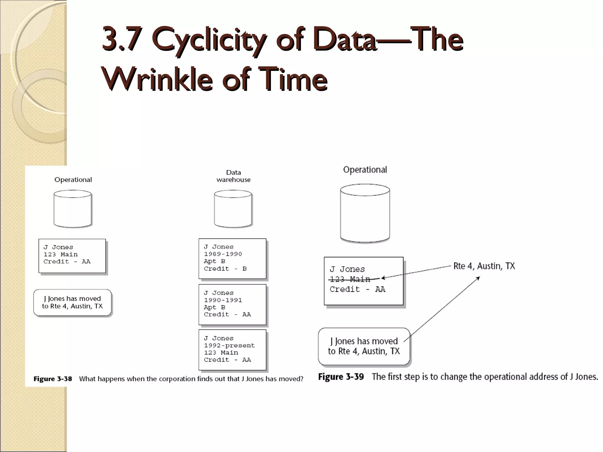
3.7 Cyclicity of Data—The
Wrinkle of Time
3.7 Cyclicity of Data—The
Wrinkle of Time (ct)
3.7 Cyclicity of Data—The
Wrinkle of Time (ct)
3.8 Complexity of Transformation
and Integration
As data passes from the operational, legacy
 environment to the data warehouse
 environment, requires transformations and or
 change in technologies
Extraction data from different sourcing systems
Transformation encoding rules and data types
Loading to new environment
3.8 Complexity of Transformation
and Integration (ct)
 ◦ The selection of data from the operational
   environment may be very complex.
 ◦ Operational input keys usually must be restructured
   and converted before they are written out to the
   data warehouse.
 ◦ Nonkey data is reformatted as it passes from the
   operational environment to the data warehouse
   environment.
    As a simple example, input data about a date is read as
     YYYY/MM/DD and is written to the output file as
     DD/MM/YYYY. (Reformatting of operational data before it is
     ready to go into a data warehouse often becomes much more
     complex than this simple example.)
3.8 Complexity of Transformation
and Integration (ct)
 ◦ Data is cleansed as it passes from the operational environment
   to the data warehouse environment.
 ◦ Multiple input sources of data exist and must be merged as they
   pass into the data warehouse.
 ◦ When there are multiple input files, key resolution must be
   done before the files can be merged.
 ◦ With multiple input files, the sequence of the files may not be
   the same or even compatible.
 ◦ Multiple outputs may result. Data may be produced at different
   levels of summarization by the same data warehouse creation
   program.
3.8 Complexity of Transformation
and Integration (ct)
 ◦ Default values must be supplied.
 ◦ The efficiency of selection of input data for
   extraction often becomes a real issue.
 ◦ Summarization of data is often required.
 ◦ Tracking the renaming of data elements as
   they are moved from the operational
   environment to the data warehouse.
3.8 Complexity of Transformation
and Integration (ct)
The    input record type conversion
 ◦   Fixed-length records
 ◦   Variable-length records
 ◦   Occurs depending on
 ◦   Occurs clause
Understand   semantic (logical meanings)
 data relationship of old systems
3.8 Complexity of Transformation
and Integration (ct)
 ◦ Data format conversion must be done.
   EBCDIC to ASCII (or vice versa) must be
   spelled out.
 ◦ Massive volumes of input must be accounted
   for.
 ◦ The design of the data warehouse must
   conform to a corporate data model.
3.8 Complexity of Transformation
and Integration (ct)
 ◦ The data warehouse reflects the historical need for
   information, while the operational environment
   focuses on the immediate, current need for
   information.
 ◦ The data warehouse addresses the informational
   needs of the corporation, while the operational
   environment addresses the up-to-the-second clerical
   needs of the corporation.
 ◦ Transmission of the newly created output file that
   will go into the data warehouse must be accounted
   for.
3.9 Triggering the Data
Warehouse Record
The  basic business interaction that populated
 data warehouse is called an event-snapshot
 interaction.
3.9.2 Components of the
Snapshot
The snapshot placed in the data warehouse normally
  contains several components.
 The unit of time that marks the occurrence of the event.
 The key that identifies the snapshot.
 The primary (nonkey) data that relates to the key
 Artifact of the relationship (secondary data that has been
  incidentally captured as of the moment of the taking of
  the snapshot and placed in the snapshot)
3.9.3 Some Examples
businessactivity might be found in a
 customer file.
The premium payments on an insurance
 policy.
3.10 Profile Records (sample)
The aggregation of operational data into a single data warehouse
  record may take many forms, including the following:
 Values taken from operational data can be summarized.
 Units of operational data can be tallied, where the total number of
  units is captured.
 Units of data can be processed to find the highest, lowest, average,
  and so forth.
 First and last occurrences of data can be trapped.
 Data of certain types, falling within the boundaries of several
  parameters, can be measured.
 Data that is effective as of some moment in time can be trapped.
 The oldest and the youngest data can be trapped.
3.10 Profile Records (ct)
3.11 Managing Volume
3.12 Creating Multiple Profile
Records
Individual   call records can be used to
 create:
 ◦ A customer profile record
 ◦ A district traffic profile record
 ◦ A line analysis profile record so forth.
3.13 Going from the Data Warehouse
to the Operational Environment
3.14 Direct Operational Access
of Data Warehouse Data
3.14 Direct Operational Access of
Data Warehouse Data (Issues)
Data  Latency (data from one source may
 not be ready for loading)
Data Volume (sizing)
Different technologies (DMBS, flatfiles,
 etc)
Different format or encoding rules
3.15 Indirect Access of Data
Warehouse Data (solution)
One  of the most effective uses of the
 data warehouse is the indirect access of
 data warehouse data by the operational
 environment
3.15.1 An Airline Commission Calculation
        System (Operational example)
The customer requests a ticket and   The airline clerk must enter and
  the travel agent wants to know       complete several transactions:
 Is there a seat available?          Are there any seats available?
 What is the cost of the seat?       Is seating preference available?
 What is the commission paid to      What connecting flights are
  the travel agent?                    involved?
                                      Can the connections be made?
                                      What is the cost of the ticket?
                                      What is the commission?
3.15.1 An Airline Commission
Calculation System (ct)
3.15.2 A Retail Personalization
       System
The retail sales representative   While engaging the customer
  could find out some other         in conversation, the sales
  information about cust.           representative may initiates
                                   “I see it’s been since
 The last type of purchase
                                    February that we last heard
  made                              from you.”
 The market segment or            “How was that blue
  segments in which the             sweater you purchased?”
  customer belongs                 “Did the problems you had
                                    with the pants get
                                    resolved?”
3.15.2 A Retail Personalization System
         (Demographics/Personalization data)
In addition, the retail sales clerk has   Retail sales representative is able to
   market segment information               ask pointed questions, such as
   available, such as the following:        these:
 Male/female                              “Did you know we have an
 Professional/other                        unannounced sale on swimsuits?”
 City/country                             “We just got in some Italian
 Children
                                            sunglasses that I think you might
                                            like.”
 Ages                                     “The forecasters predict a cold
 Sex                                       winter for duck hunters. We
 Sports                                    have a special on waders right
 Fishing                                   now.”
 Hunting
 Beach
3.15.2 A Retail Personalization
System (ct)
3.15.2 A Retail Personalization
System (ct)
Periodically, the analysis program spins off
 a file to the operational environment that
 contains such information as the
 following:
Last purchase date
Last purchase type
Market analysis/segmenting
3.15.3 Credit Scoring
based on (Demographics data)
The background check relies on the data warehouse. In
  truth, the check is an eclectic one, in which many
  aspects of the customer are investigated, such as the
  following:
 Past payback history
 Home/property ownership
 Financial management
 Net worth
 Gross income
 Gross expenses
 Other intangibles
3.15.3 Credit Scoring (ct)
The analysis program is run periodically
 and produces a prequalified file for use in
 the operational environment. In addition
 to other data, the prequalified file
 includes the following:
Customer identification
Approved credit limit
Special approval limit
3.15.3 Credit Scoring (ct)
3.16 Indirect Use of Data
Warehouse Data
3.16 Indirect Use of Data
Warehouse Data (ct)
Following are a few considerations of the elements of the indirect use
  of data warehouse data:
 The analysis program:
    ◦ Has many characteristics of artificial intelligence
    ◦ Has free rein to run on any data warehouse data that is available
    ◦ Is run in the background, where processing time is not an issue (or at
      least not a large issue)
    ◦ Is run in harmony with the rate at which data warehouse changes
   The periodic refreshment:
    ◦ Occurs infrequently
    ◦ Operates in a replacement mode
    ◦ Moves the data from the technology supporting the data warehouse to
      the technology supporting the operational environment
3.16 Indirect Use of Data
Warehouse Data (ct)
The   online pre-analyzed data file:
 ◦ Contains only a small amount of data per unit of data
 ◦ May contain collectively a large amount of data
   (because there may be many units of data)
 ◦ Contains precisely what the online clerk needs
 ◦ Is not updated, but is periodically refreshed on a
   wholesale basis
 ◦ Is part of the online high-performance environment
 ◦ Is efficient to access
 ◦ Is geared for access of individual units of data, not
   massive sweeps of data
3.17 Star Joins
There are several very good reasons why
 normalization and a relational approach
 produces the optimal design for a data
 warehouse:
It produces flexibility.
It fits well with very granular data.
It is not optimized for any given set of
 processing requirements.
It fits very nicely with the data model.
3.17 Star Joins (ct)
3.18 Supporting the ODS
In general, there are four classes of ODS:
 Class I—In a class I ODS, updates of data from the operational
   environment to the ODS are synchronous.
 Class II— In a class II ODS, the updates between the operational
   environment and the ODS occur within a two-to-three-hour time
   frame.
 Class III—In a class III ODS, the synchronization of updates
   between the operational environment and the ODS occurs
   overnight.
 Class IV—In a class IV ODS, updates into the ODS from the data
   warehouse are unscheduled. Figure 3-56 shows this support.
3.18 Supporting the ODS (ct)
The customer has been active for several years. The
  analysis of the transactions in the data warehouse is
  used to produce the following profile information about
  a single customer:
 Customer name and ID
 Customer volume—high/low
 Customer profitability—high/low
 Customer frequency of activity—very frequent/very
  infrequent
 Customer likes/dislikes (fast cars, single malt scotch)
3.18 Supporting the ODS (ct)
3.19 Requirements and the
Zachman Framework
3.19 Requirements and the
Zachman Framework (ct)
Summary
   Design of data warehouse
    ◦   Corporate Data model
    ◦   Operational data model
    ◦   Iterative approach since requirements are a non-priori
    ◦   Different SDLC approach
   Data warehouse construction considerations
    ◦ Data Volume (large size)
    ◦ Data Latency (late arrival of data set)
    ◦ Require transformation and understand of legacy
   Data Models (granularities)
    ◦ Low level
    ◦ Mid Level
    ◦ High Level
   Structure of typical record in data warehouse
    ◦ Time stamp, a surrogate key, direct data, secondary data
Summary
(cont’)
     Reference   tables must be manage in time-variant
      manner
     Data Latency – wrinkles of time
     Data Transformation is complex
      ◦ Different architectures
      ◦ Different technologies
      ◦ Different encoding rules and complex logics
     Creation   of data warehouse record is triggered by on
      event (activity)
     A profile record is a composite representation of data
      (historical activities)
     Star Join (is a preferred database design techniques


                       Visit us : http://it-slideshares.blogspot.com/

Lecture 03 - The Data Warehouse and Design

  • 1.
    Building Data Warehouse ByInmon Chapter 3: The Data Warehouse and Design
  • 2.
    3.0 Introduction There aretwo major components to building a data warehouse: The design of the interface from operational systems. The design of the data warehouse itself.
  • 3.
    3.1 Beginning withOperational Data  Design begins with the considerations of placing data in the data warehouse.
  • 4.
    3.1 Beginning withOperational Data (Different applications integration)
  • 5.
    3.1 Beginning withOperational Data (Encoding Transformation)
  • 6.
    3.1 Beginning withOperational Data ( Types of Data Load) Three types of loads are made into the data warehouse from the operational environment: Archival data Data currently contained in the operational environment Ongoing changes to the data warehouse environment from the changes (updates) that have occurred in the operational environment since the last refresh
  • 7.
    3.1 Beginning withOperational Data (Data selection)
  • 8.
    3.1 Beginning withOperational Data (Data Selection – time based)
  • 9.
    3.1 Beginning withOperational Data (Data Selection: spatial consideration)
  • 10.
    3.2 Process andData Models and the Architected Environment
  • 11.
    3.2 Process andData Models and the Architected Environment (ct) Data models are discussed in depth in the following section. 1. Functional decomposition 2. Context-level zero diagram 3. Data flow diagram 4. Structure chart 5. State transition diagram 6. HIPO chart 7. Pseudo code
  • 12.
    3.3 The DataWarehouse and Data Models
  • 13.
    3.3 The DataWarehouse and Data Models (ct)
  • 14.
    3.3.1 The DataWarehouse Data Model
  • 15.
    3.3.1 The DataWarehouse Data Model (ct)
  • 16.
    3.3.1 The DataWarehouse Data Model (ct)
  • 17.
  • 18.
    3.3.2 The MidlevelData Model (ct) Four basic constructs are found at the midlevel model:  A primary grouping of data —The primary grouping exists once, and only once, for each major subject area. It holds attributes that exist only once for each major subject area. As with all groupings of data, the primary grouping contains attributes and keys for each major subject area.  A secondary grouping of data —The secondary grouping holds data attributes that can exist multiple times for each major subject area. This grouping is indicated by a line emanating downward from the primary grouping of data. There may be as many secondary groupings as there are distinct groups of data that can occur multiple times.  A connector—This signifies the relationships of data between major subject areas. The connector relates data from one grouping to another. A relationship identified at the ERD level results in an acknowledgment at the DIS level. The convention used to indicate a connector is an underlining of a foreign key.  “Type of” data —This data is indicated by a line leading to the right of a grouping of data. The grouping of data to the left is the supertype. The grouping of data to the right is the subtype of data.
  • 19.
    3.3.2 The MidlevelData Model (ct)
  • 20.
    3.3.2 The MidlevelData Model (ct)
  • 21.
    3.3.2 The MidlevelData Model (ct)
  • 22.
    3.3.2 The MidlevelData Model (ct) Of particular interest is the case where a grouping of data has two “type of” lines emanating from it, as shown in Figure 3-17. The two lines leading to the right indicate that there are two “type of” criteria. One type of criteria is by activity type—either a deposit or a withdrawal. The other line indicates another activity type—either an ATM activity or a teller activity. Collectively, the two types of activity encompass the following transactions:  ATM deposit  ATM withdrawal  Teller deposit  Teller withdrawal
  • 23.
    3.3.2 The MidlevelData Model (ct) The physical table entries that resulted came from the following two transactions: An ATM withdrawal that occurred at 1:31 p.m. on January 2 A teller deposit that occurred at 3:15 p.m. on January 5
  • 24.
    3.3.2 The MidlevelData Model (ct)
  • 25.
  • 26.
    3.3.3 The PhysicalData Model (ct)
  • 27.
    3.3.3 The PhysicalData Model (con’t)
  • 28.
    3.3.3 The PhysicalData Model (con’t)
  • 29.
    3.3.3 The PhysicalData Model (con’t) Note: This is not an issue of blindly transferring a large number of records from DASD to main storage. Instead, it is a more sophisticated issue of transferring a bulk of records that have a high probability of being accessed.
  • 30.
    3.4 The DataModel and Iterative Development Why iterative development is important ? The industry track record of success strongly suggests it. The end user is unable to articulate many requirements until the first iteration is done. Management will not make a full commitment until at least a few actual results are tangible and obvious. Visible results must be seen quickly.
  • 31.
    3.4 The DataModel and Iterative Development (ct)
  • 32.
    3.4 The DataModel and Iterative Development (ct)
  • 33.
    3.5 Normalization andDenormalization (ERD: Entity Relationship Diagram)
  • 34.
    3.5 Normalization andDenormalization (Dimensional Modeling Technique)
  • 35.
    3.5 Normalization andDenormalization (hash algorithm: better search ability)
  • 36.
    3.5 Normalization andDenormalization (Use of Redundancy data – search performance)
  • 37.
    3.5 Normalization andDenormalization (Separation of data & access probability)
  • 38.
    3.5 Normalization andDenormalization (Derived Data – What is it ?)
  • 39.
    3.5 Normalization andDenormalization (Data Indexing vs. Profiles – Why ?)
  • 40.
    3.5 Normalization andDenormalization (Referential data Integrity)
  • 41.
    3.5.1 Snapshots inthe Data Warehouse The snapshot triggered by an event has four basic components: A key A unit of time Primary data that relates only to the key Secondary data captured as part of the snapshot process that has no direct relationship to the primary data or key
  • 42.
    3.5.1 Snapshots inthe Data Warehouse (Primary Data)
  • 43.
    3.5.1 Snapshots inthe Data Warehouse (Primary & 2nd data)
  • 44.
    3.6 Metadata Metadata sitsabove the warehouse and keeps track of what is where in the warehouse such as:  Structure of data as known to the programmer  Structure of data as known to the DSS analyst  Source data feeding the data warehouse  Transformation of data as it passes into the data warehouse  Data model  Relationship between the data model and the data warehouse  History of extracts
  • 45.
    3.6.1 Managing ReferenceTables in a Data Warehouse
  • 46.
    3.6.1 Managing ReferenceTables in a Data Warehouse (ct)
  • 47.
    3.7 Cyclicity ofData—The Wrinkle of Time
  • 48.
    3.7 Cyclicity ofData—The Wrinkle of Time (ct)
  • 49.
    3.7 Cyclicity ofData—The Wrinkle of Time (ct)
  • 50.
    3.8 Complexity ofTransformation and Integration As data passes from the operational, legacy environment to the data warehouse environment, requires transformations and or change in technologies Extraction data from different sourcing systems Transformation encoding rules and data types Loading to new environment
  • 51.
    3.8 Complexity ofTransformation and Integration (ct) ◦ The selection of data from the operational environment may be very complex. ◦ Operational input keys usually must be restructured and converted before they are written out to the data warehouse. ◦ Nonkey data is reformatted as it passes from the operational environment to the data warehouse environment.  As a simple example, input data about a date is read as YYYY/MM/DD and is written to the output file as DD/MM/YYYY. (Reformatting of operational data before it is ready to go into a data warehouse often becomes much more complex than this simple example.)
  • 52.
    3.8 Complexity ofTransformation and Integration (ct) ◦ Data is cleansed as it passes from the operational environment to the data warehouse environment. ◦ Multiple input sources of data exist and must be merged as they pass into the data warehouse. ◦ When there are multiple input files, key resolution must be done before the files can be merged. ◦ With multiple input files, the sequence of the files may not be the same or even compatible. ◦ Multiple outputs may result. Data may be produced at different levels of summarization by the same data warehouse creation program.
  • 53.
    3.8 Complexity ofTransformation and Integration (ct) ◦ Default values must be supplied. ◦ The efficiency of selection of input data for extraction often becomes a real issue. ◦ Summarization of data is often required. ◦ Tracking the renaming of data elements as they are moved from the operational environment to the data warehouse.
  • 54.
    3.8 Complexity ofTransformation and Integration (ct) The input record type conversion ◦ Fixed-length records ◦ Variable-length records ◦ Occurs depending on ◦ Occurs clause Understand semantic (logical meanings) data relationship of old systems
  • 55.
    3.8 Complexity ofTransformation and Integration (ct) ◦ Data format conversion must be done. EBCDIC to ASCII (or vice versa) must be spelled out. ◦ Massive volumes of input must be accounted for. ◦ The design of the data warehouse must conform to a corporate data model.
  • 56.
    3.8 Complexity ofTransformation and Integration (ct) ◦ The data warehouse reflects the historical need for information, while the operational environment focuses on the immediate, current need for information. ◦ The data warehouse addresses the informational needs of the corporation, while the operational environment addresses the up-to-the-second clerical needs of the corporation. ◦ Transmission of the newly created output file that will go into the data warehouse must be accounted for.
  • 57.
    3.9 Triggering theData Warehouse Record The basic business interaction that populated data warehouse is called an event-snapshot interaction.
  • 58.
    3.9.2 Components ofthe Snapshot The snapshot placed in the data warehouse normally contains several components.  The unit of time that marks the occurrence of the event.  The key that identifies the snapshot.  The primary (nonkey) data that relates to the key  Artifact of the relationship (secondary data that has been incidentally captured as of the moment of the taking of the snapshot and placed in the snapshot)
  • 59.
    3.9.3 Some Examples businessactivitymight be found in a customer file. The premium payments on an insurance policy.
  • 60.
    3.10 Profile Records(sample) The aggregation of operational data into a single data warehouse record may take many forms, including the following:  Values taken from operational data can be summarized.  Units of operational data can be tallied, where the total number of units is captured.  Units of data can be processed to find the highest, lowest, average, and so forth.  First and last occurrences of data can be trapped.  Data of certain types, falling within the boundaries of several parameters, can be measured.  Data that is effective as of some moment in time can be trapped.  The oldest and the youngest data can be trapped.
  • 61.
  • 62.
  • 63.
    3.12 Creating MultipleProfile Records Individual call records can be used to create: ◦ A customer profile record ◦ A district traffic profile record ◦ A line analysis profile record so forth.
  • 64.
    3.13 Going fromthe Data Warehouse to the Operational Environment
  • 65.
    3.14 Direct OperationalAccess of Data Warehouse Data
  • 66.
    3.14 Direct OperationalAccess of Data Warehouse Data (Issues) Data Latency (data from one source may not be ready for loading) Data Volume (sizing) Different technologies (DMBS, flatfiles, etc) Different format or encoding rules
  • 67.
    3.15 Indirect Accessof Data Warehouse Data (solution) One of the most effective uses of the data warehouse is the indirect access of data warehouse data by the operational environment
  • 68.
    3.15.1 An AirlineCommission Calculation System (Operational example) The customer requests a ticket and The airline clerk must enter and the travel agent wants to know complete several transactions:  Is there a seat available?  Are there any seats available?  What is the cost of the seat?  Is seating preference available?  What is the commission paid to  What connecting flights are the travel agent? involved?  Can the connections be made?  What is the cost of the ticket?  What is the commission?
  • 69.
    3.15.1 An AirlineCommission Calculation System (ct)
  • 70.
    3.15.2 A RetailPersonalization System The retail sales representative While engaging the customer could find out some other in conversation, the sales information about cust. representative may initiates  “I see it’s been since  The last type of purchase February that we last heard made from you.”  The market segment or  “How was that blue segments in which the sweater you purchased?” customer belongs  “Did the problems you had with the pants get resolved?”
  • 71.
    3.15.2 A RetailPersonalization System (Demographics/Personalization data) In addition, the retail sales clerk has Retail sales representative is able to market segment information ask pointed questions, such as available, such as the following: these:  Male/female  “Did you know we have an  Professional/other unannounced sale on swimsuits?”  City/country  “We just got in some Italian  Children sunglasses that I think you might like.”  Ages  “The forecasters predict a cold  Sex winter for duck hunters. We  Sports have a special on waders right  Fishing now.”  Hunting  Beach
  • 72.
    3.15.2 A RetailPersonalization System (ct)
  • 73.
    3.15.2 A RetailPersonalization System (ct) Periodically, the analysis program spins off a file to the operational environment that contains such information as the following: Last purchase date Last purchase type Market analysis/segmenting
  • 74.
    3.15.3 Credit Scoring basedon (Demographics data) The background check relies on the data warehouse. In truth, the check is an eclectic one, in which many aspects of the customer are investigated, such as the following:  Past payback history  Home/property ownership  Financial management  Net worth  Gross income  Gross expenses  Other intangibles
  • 75.
    3.15.3 Credit Scoring(ct) The analysis program is run periodically and produces a prequalified file for use in the operational environment. In addition to other data, the prequalified file includes the following: Customer identification Approved credit limit Special approval limit
  • 76.
  • 77.
    3.16 Indirect Useof Data Warehouse Data
  • 78.
    3.16 Indirect Useof Data Warehouse Data (ct) Following are a few considerations of the elements of the indirect use of data warehouse data:  The analysis program: ◦ Has many characteristics of artificial intelligence ◦ Has free rein to run on any data warehouse data that is available ◦ Is run in the background, where processing time is not an issue (or at least not a large issue) ◦ Is run in harmony with the rate at which data warehouse changes  The periodic refreshment: ◦ Occurs infrequently ◦ Operates in a replacement mode ◦ Moves the data from the technology supporting the data warehouse to the technology supporting the operational environment
  • 79.
    3.16 Indirect Useof Data Warehouse Data (ct) The online pre-analyzed data file: ◦ Contains only a small amount of data per unit of data ◦ May contain collectively a large amount of data (because there may be many units of data) ◦ Contains precisely what the online clerk needs ◦ Is not updated, but is periodically refreshed on a wholesale basis ◦ Is part of the online high-performance environment ◦ Is efficient to access ◦ Is geared for access of individual units of data, not massive sweeps of data
  • 80.
    3.17 Star Joins Thereare several very good reasons why normalization and a relational approach produces the optimal design for a data warehouse: It produces flexibility. It fits well with very granular data. It is not optimized for any given set of processing requirements. It fits very nicely with the data model.
  • 81.
  • 82.
  • 83.
  • 84.
  • 85.
  • 86.
  • 87.
  • 88.
  • 89.
    3.18 Supporting theODS In general, there are four classes of ODS:  Class I—In a class I ODS, updates of data from the operational environment to the ODS are synchronous.  Class II— In a class II ODS, the updates between the operational environment and the ODS occur within a two-to-three-hour time frame.  Class III—In a class III ODS, the synchronization of updates between the operational environment and the ODS occurs overnight.  Class IV—In a class IV ODS, updates into the ODS from the data warehouse are unscheduled. Figure 3-56 shows this support.
  • 90.
    3.18 Supporting theODS (ct) The customer has been active for several years. The analysis of the transactions in the data warehouse is used to produce the following profile information about a single customer:  Customer name and ID  Customer volume—high/low  Customer profitability—high/low  Customer frequency of activity—very frequent/very infrequent  Customer likes/dislikes (fast cars, single malt scotch)
  • 91.
  • 92.
    3.19 Requirements andthe Zachman Framework
  • 93.
    3.19 Requirements andthe Zachman Framework (ct)
  • 94.
    Summary  Design of data warehouse ◦ Corporate Data model ◦ Operational data model ◦ Iterative approach since requirements are a non-priori ◦ Different SDLC approach  Data warehouse construction considerations ◦ Data Volume (large size) ◦ Data Latency (late arrival of data set) ◦ Require transformation and understand of legacy  Data Models (granularities) ◦ Low level ◦ Mid Level ◦ High Level  Structure of typical record in data warehouse ◦ Time stamp, a surrogate key, direct data, secondary data
  • 95.
    Summary (cont’)  Reference tables must be manage in time-variant manner  Data Latency – wrinkles of time  Data Transformation is complex ◦ Different architectures ◦ Different technologies ◦ Different encoding rules and complex logics  Creation of data warehouse record is triggered by on event (activity)  A profile record is a composite representation of data (historical activities)  Star Join (is a preferred database design techniques Visit us : http://it-slideshares.blogspot.com/