Downloaded 128 times

![5
Gaussian Integration
• For Newton-Cotes methods we have:
b
b −a
1. ∫ f ( x )dx ≅ [ f (a) + f (b)].
a
2
b
b −a a +b
2. ∫
b
f ( x )dx ≅
6
f (a ) + 4 f (
2
) + f (b) .
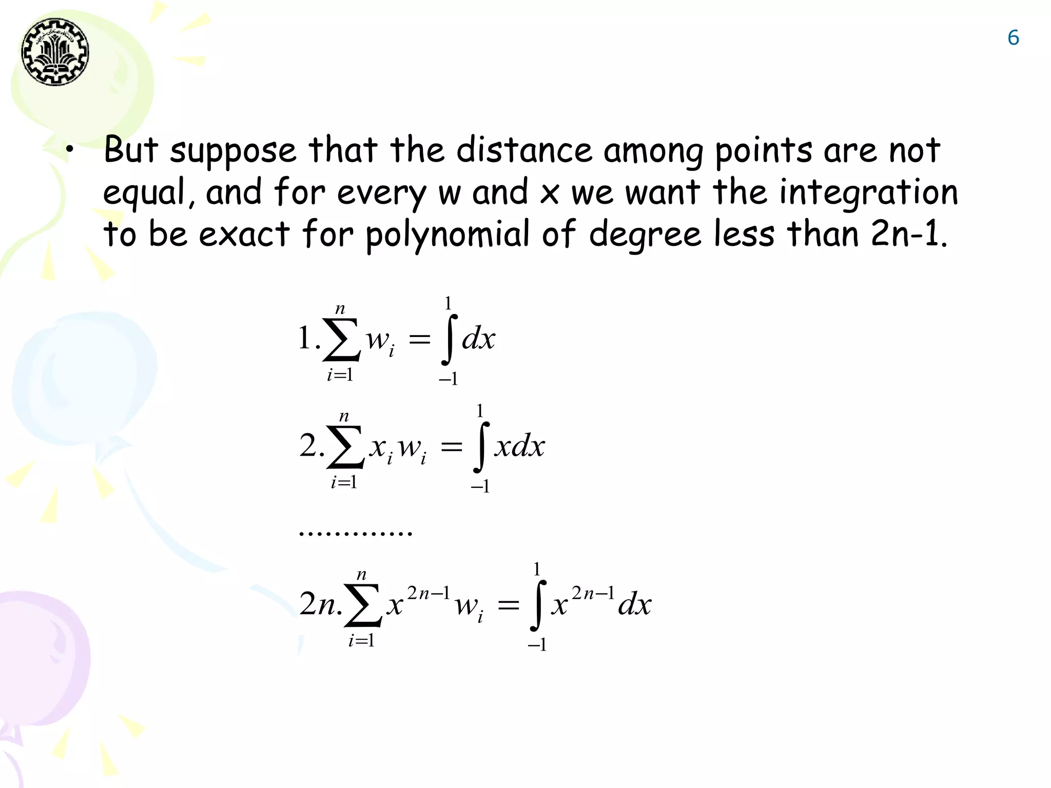
• And in general form:
b n
∫ f ( x)dx ≅ ∑ w f ( x )i i xi = a + (i − 1)h i ∈ {1,2,3,..., n}
a i =1
n
b− a n t− j
wi = ∏ dt
n − 1 ∫ j =1, j ≠ i i − j
0](https://image.slidesharecdn.com/gausianintegration-120615144049-phpapp01/75/Gaussian-Integration-5-2048.jpg)
![12
Theorem:
1 n (x − x j )
wi = ∫ [ Li ( x )] dx ∏ (x
2
Li ( x ) =
−1 j = , j ≠i
1 i −xj )
Proof:
1 2
[ Li ( x)] 2 ∈ Π 2 n−2 ⇒ ∫ [ Li ( x)] 2 = ∑ w j [ Li ( x j )]
n
= wi .
−1 j =1](https://image.slidesharecdn.com/gausianintegration-120615144049-phpapp01/75/Gaussian-Integration-12-2048.jpg)
![13
Error Analysis for
Gaussian Integration
• Error analysis for Gaussian integrals can be derived
according to Hermite Interpolation.
b
Theorem : The error made by gaussian integration in approximation the integral ∫ f ( x )dx is ::
a
(b − a ) 2 n +1 ( N !) 4
EN ( f ) = f (2n)
(ξ ) ξ ∈ [ a, b].
(2n + 1)((2n)!) 3](https://image.slidesharecdn.com/gausianintegration-120615144049-phpapp01/75/Gaussian-Integration-13-2048.jpg)
![15
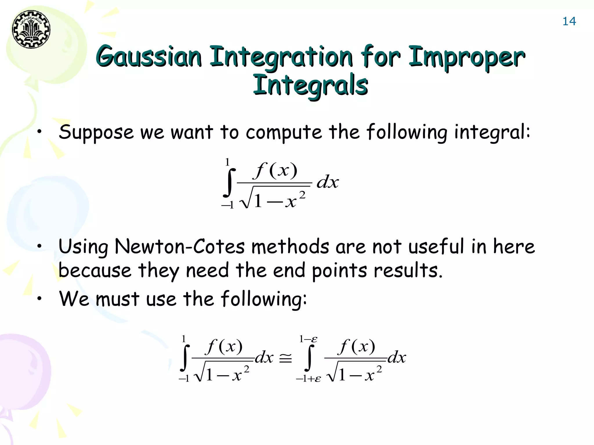
• But we can use the Gaussian formula because it does
not need the value at the endpoints.
• But according to the error of Gaussian integration,
Gaussian integration is also not proper in this case.
• We need better approach.
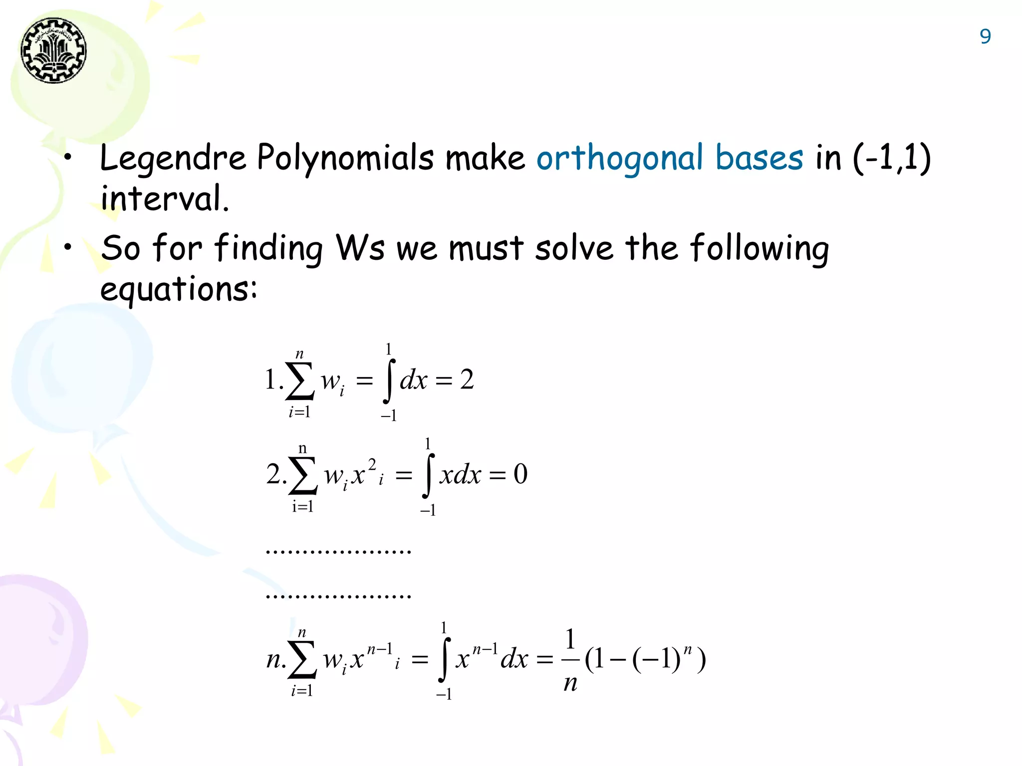
Definition : The Polynomial set { Pi } is orthogonal in (a, b) with respect to w(x) if :
b
∫ w( x) P ( x)P
a
i j ( x) dx = 0 for i ≠ j
then we have the following approximation :
b n
∫ w( x) f ( x)dx ≅ ∑ wi f ( xi )
a i =1
where xi are the roots for Pn and
b
wi = ∫ w( x)[ Li ( x)] dx
2
a
will compute the integral exactly when f ∈ Π 2 n −1](https://image.slidesharecdn.com/gausianintegration-120615144049-phpapp01/75/Gaussian-Integration-15-2048.jpg)

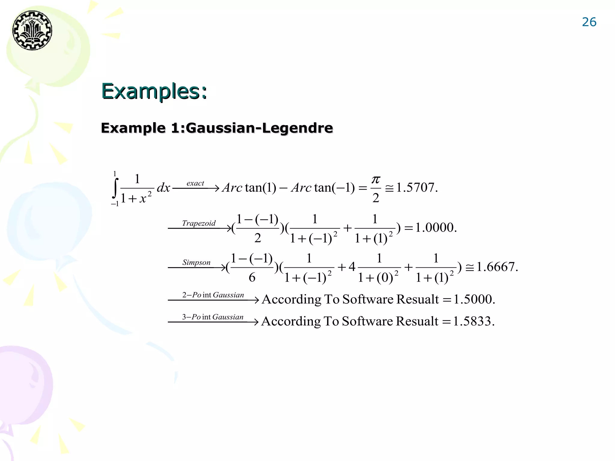
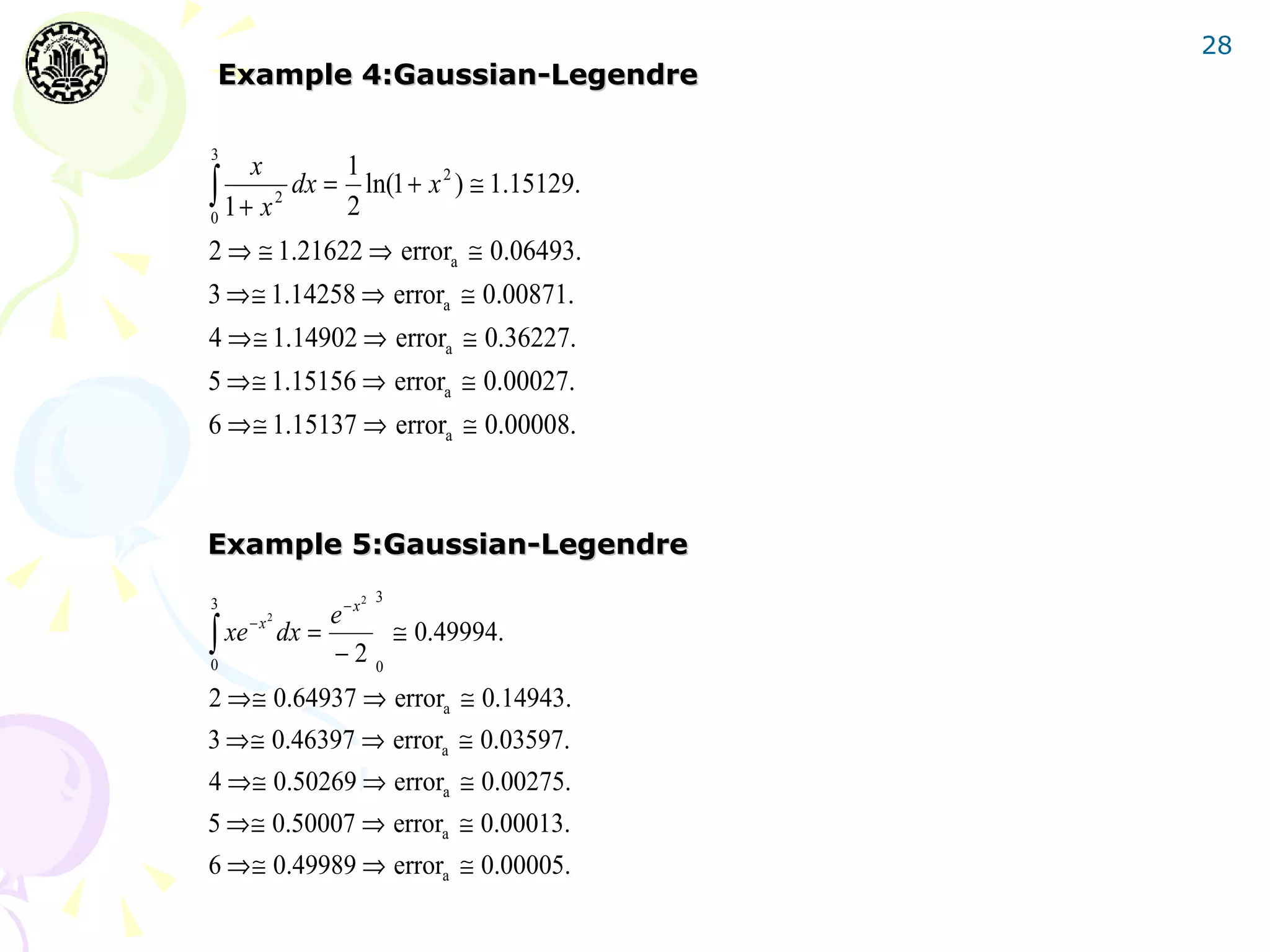
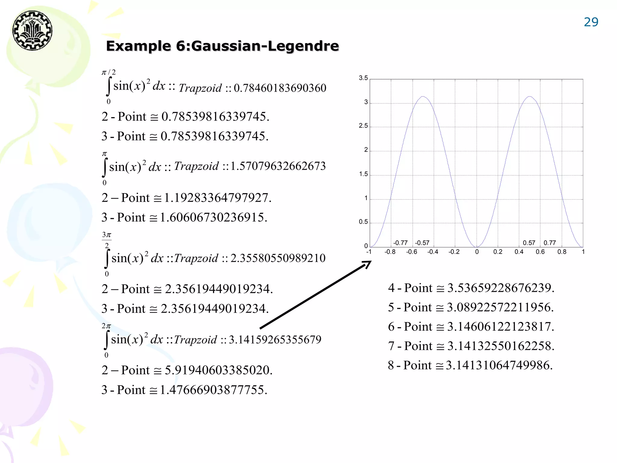
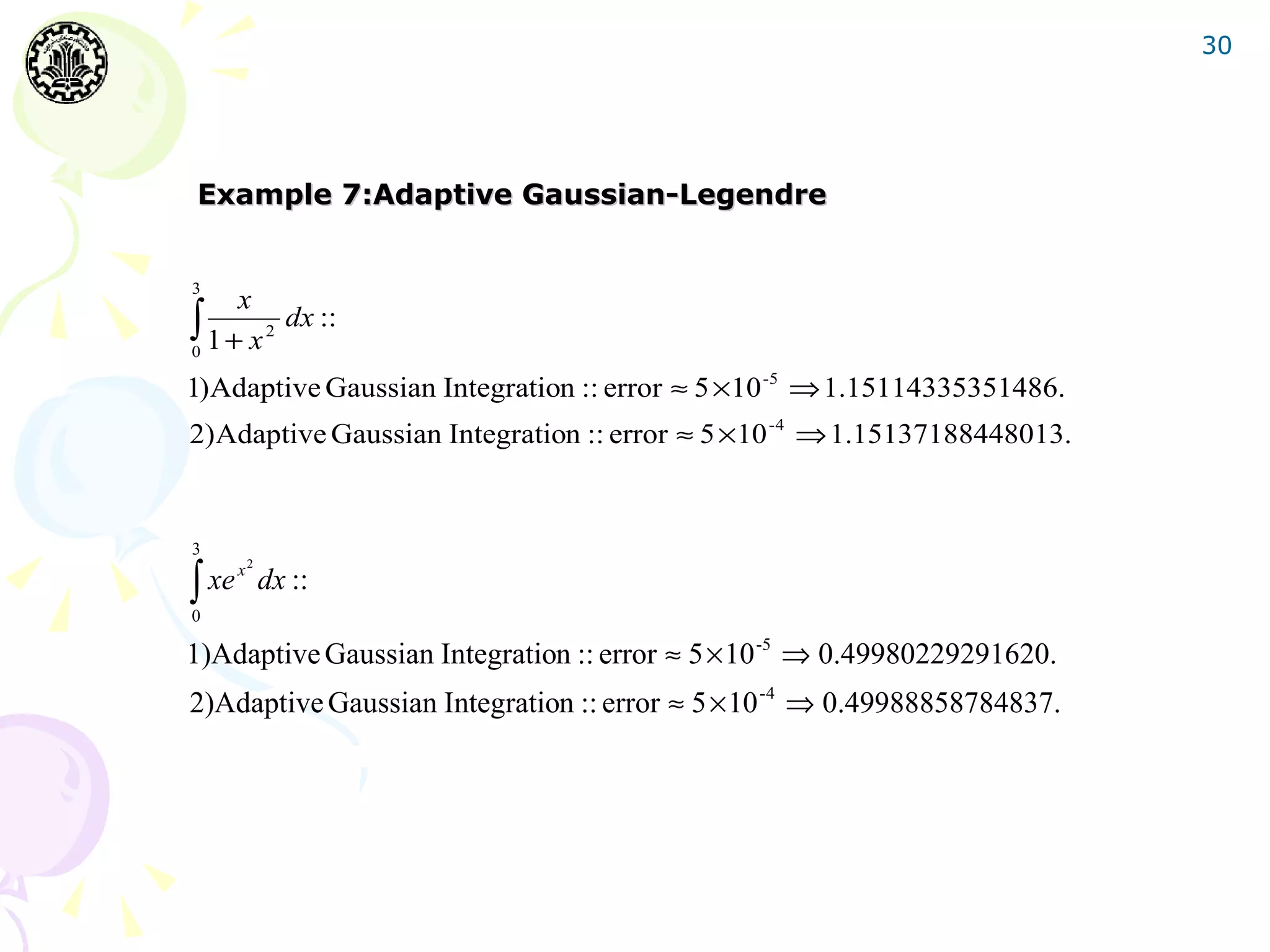
![27
Example 2:Gaussian-Legendre
2
− e−x 3 − e −9 1
3
∫ xe
2
−x
dx →(
exact
)0 = ( + ) ≅ 0.4999.
0
2 2 2
3− 0
Trapezoid →(
)(0 + 3e −9 ) ≅ 0.0005.
2
3−0 2
Simpson → (
)(0 + 1.5e −1.5 + 3e −9 ) ≅ 0.0792.
6
2− Po int Gaussian → ≅ 0.6494.
3− Po int Gaussian → ≅ 0.4640.
Example 3:Gaussian-Legendre
(b − a ) 2 n +1 ( n!) 4
En ( f ) = f 2n
(ξ ) ξ ∈[a, b].
( 2n +1)((2n)!) 3
π
(π − 0) 2 n +1 ( n!) 4
∫ sin( x)dx → | (2n +1)((2n)!) 3 sin (ξ ) |≤ 5 ×10 ⇒ n ≥ 4.
−4
2n
0
( 2 − 0) 2 n +1 (n!) 4 −ξ
2
∫ e dx →| (2n +1)((2n)!) 3 e |≤ 5 ×10 ⇒ n ≥ 3.
−x −4
0](https://image.slidesharecdn.com/gausianintegration-120615144049-phpapp01/75/Gaussian-Integration-27-2048.jpg)


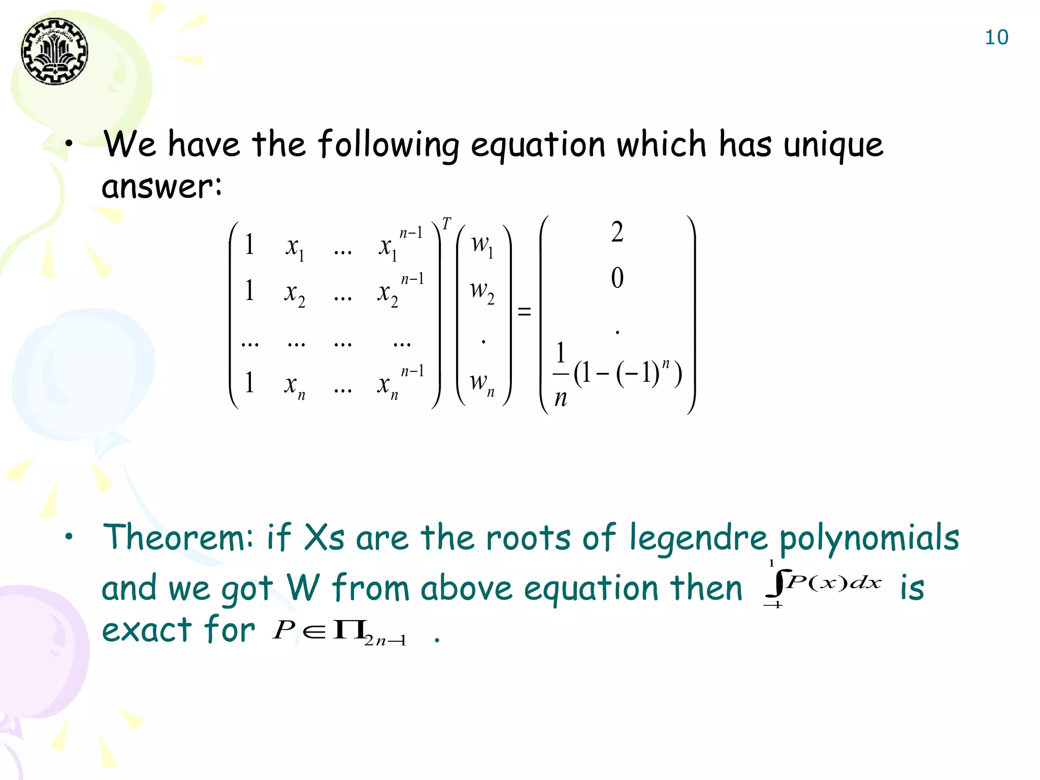
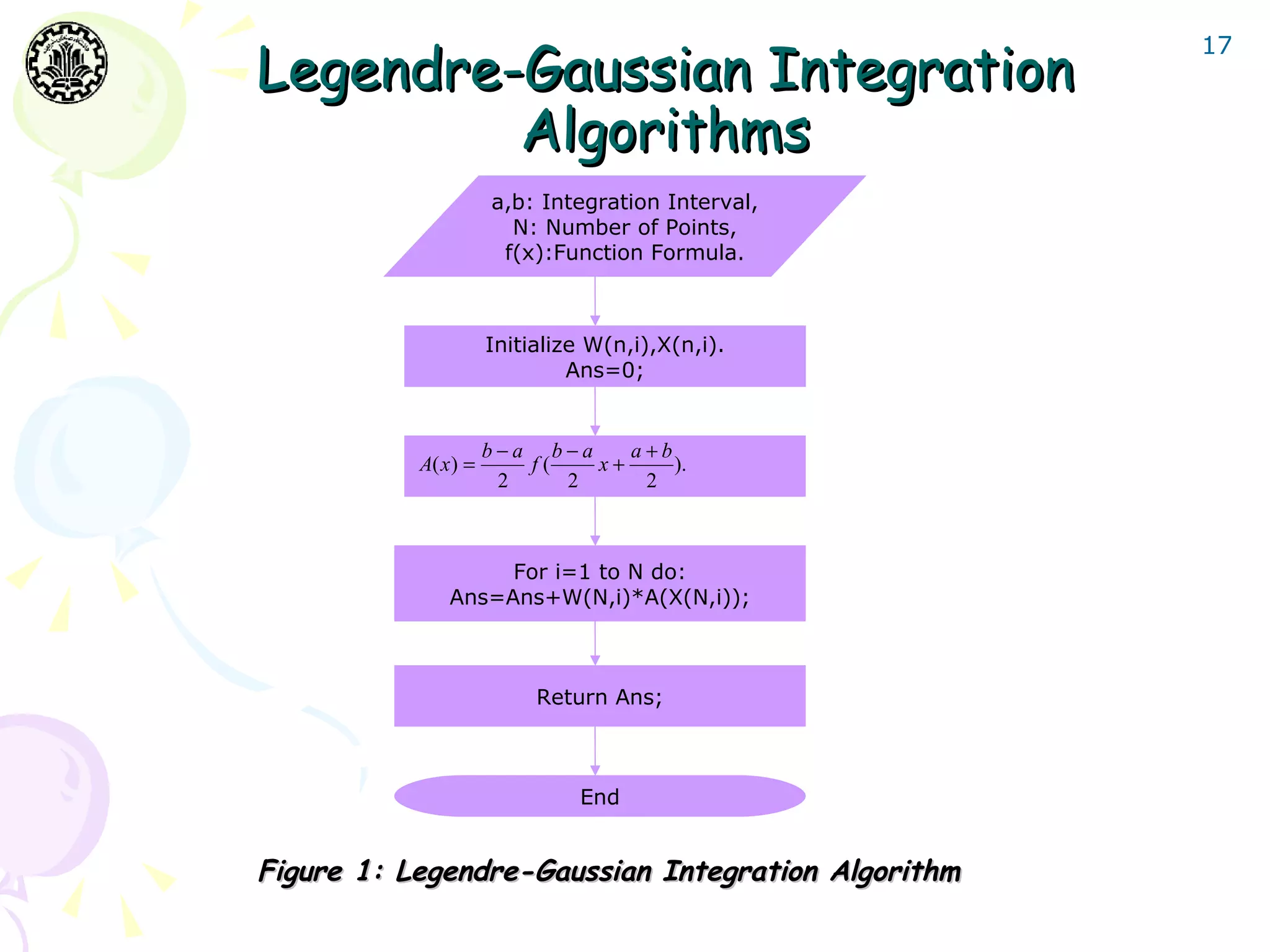
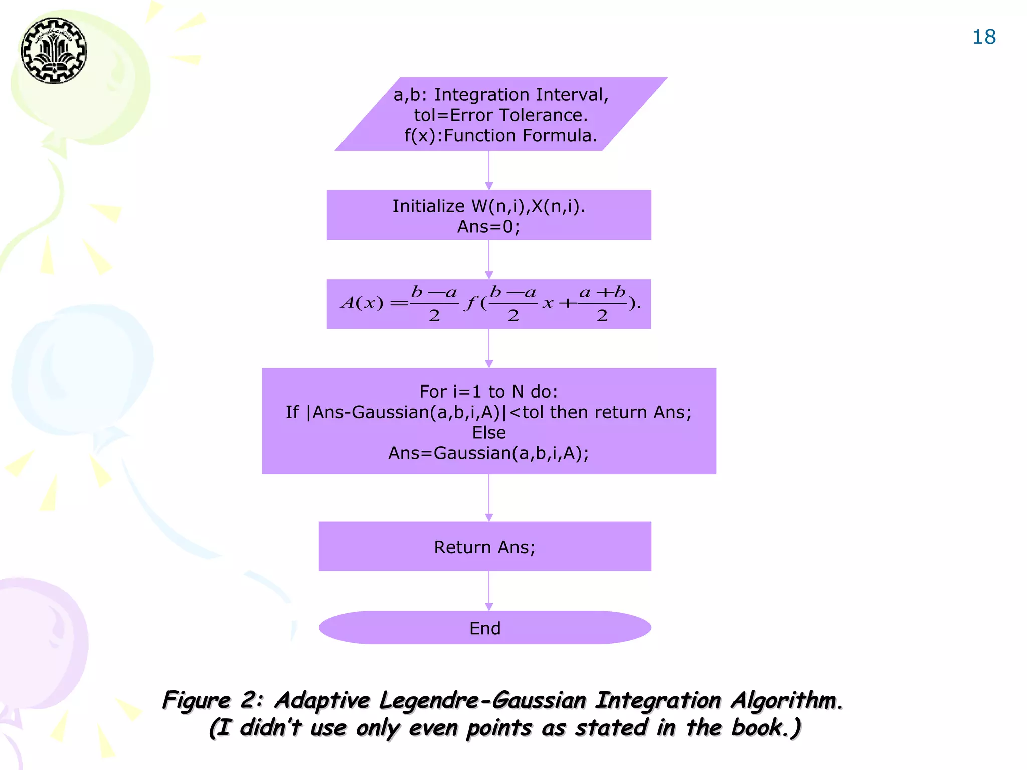
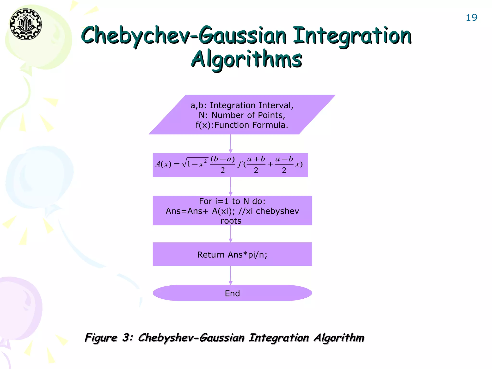
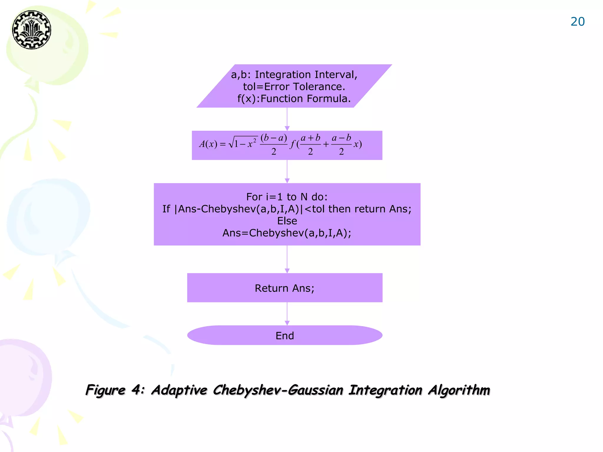
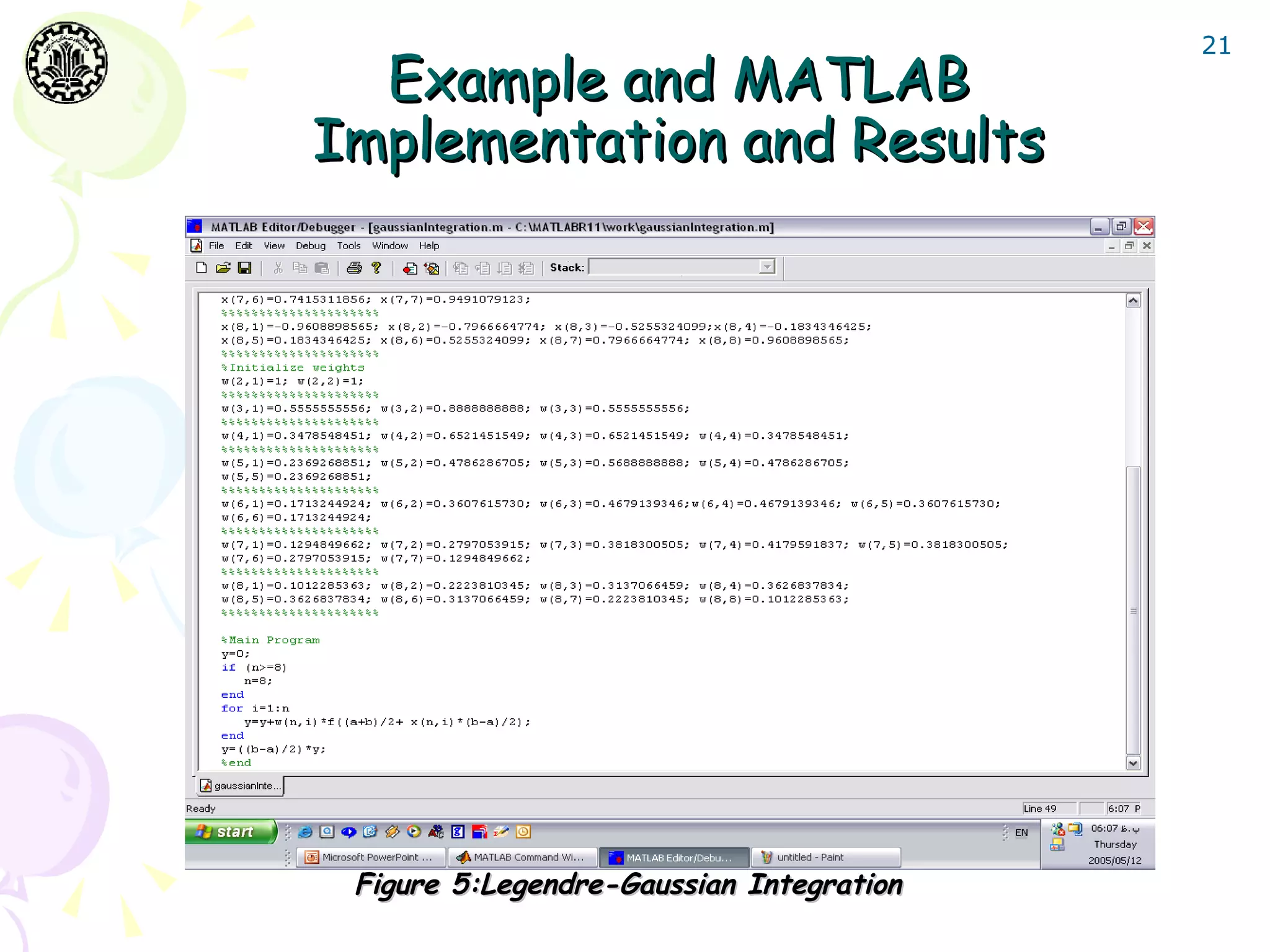
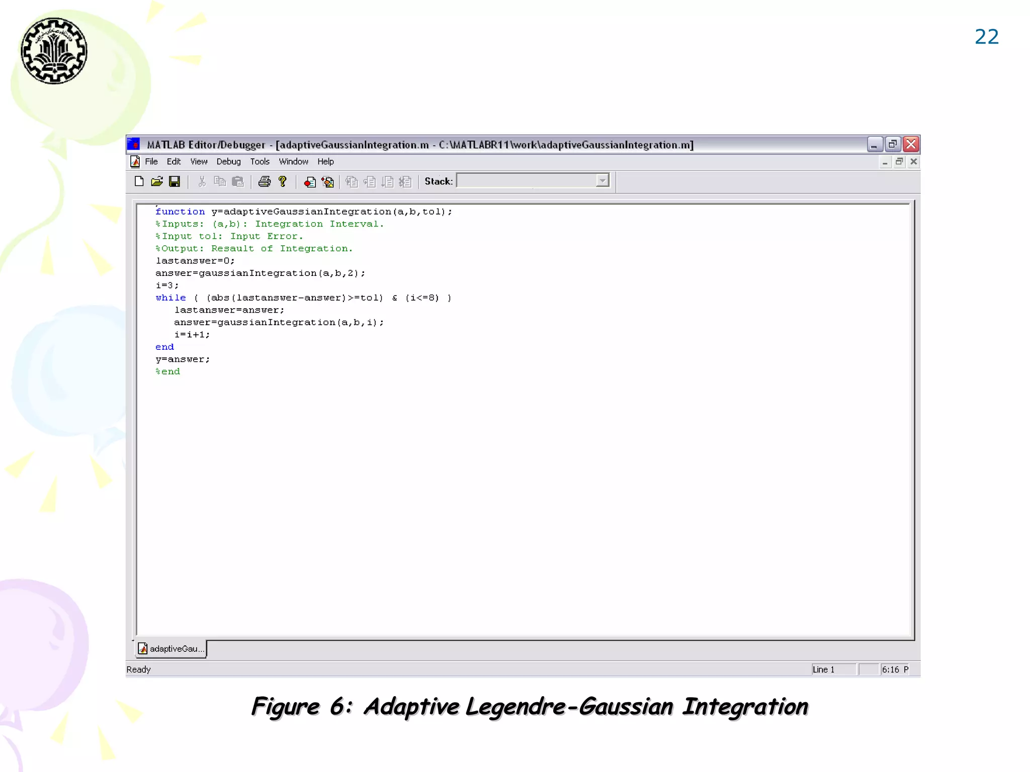
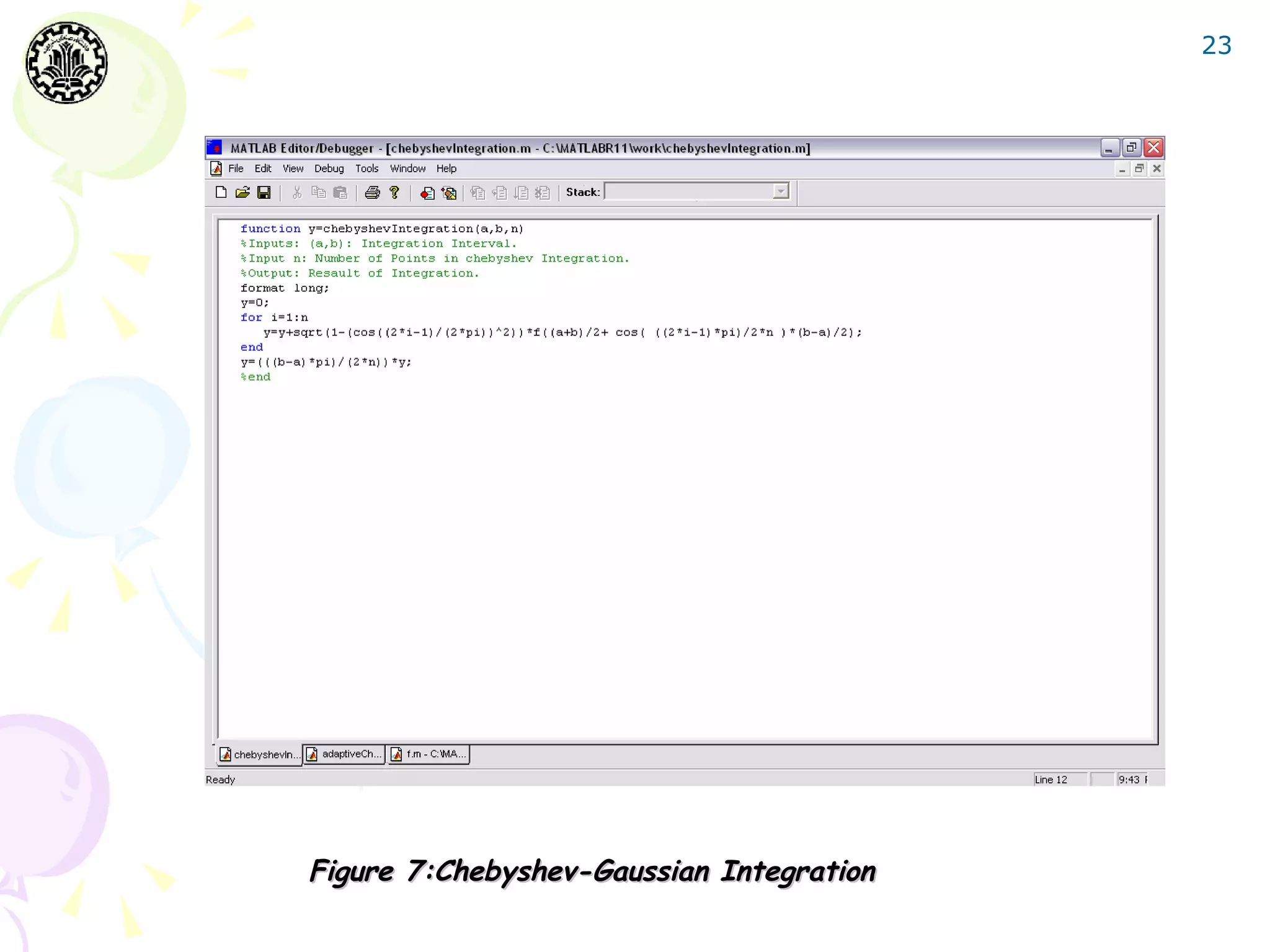
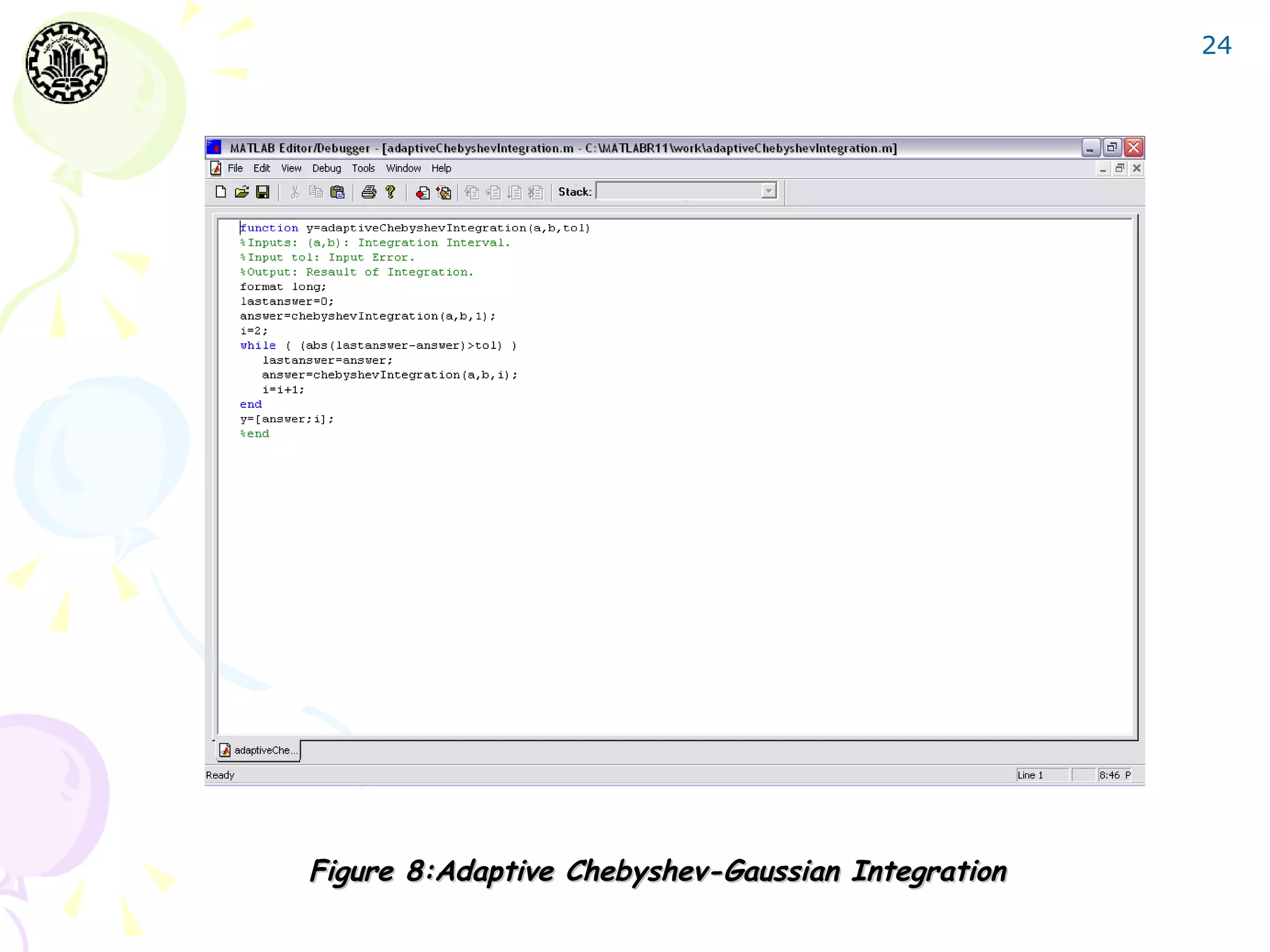
The document discusses Gaussian integration techniques, outlining their advantages over traditional methods like Newton-Cotes and Romberg integration, particularly highlighting the role of Legendre polynomials and Chebyshev polynomials in deriving Gaussian formulas for accurate numerical integration. It covers error analysis, implications for improper integrals, and provides MATLAB implementation examples with results demonstrating the effectiveness of these algorithms. Additionally, various algorithms for Legendre and Chebyshev integration are presented, alongside error tolerance considerations and sample computational results.