From the course PHYS261, University of Bergen. This is a PDF with links. The links do not work here on slideshare preview.

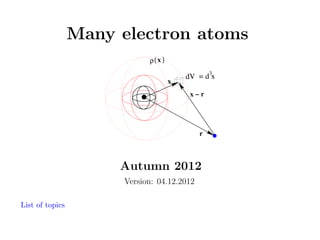
1. Many electron atoms
ρ( x )
x
3
dV = d x
x−r
r
Autumn 2012
Version: 04.12.2012
List of topics

2. (1)
Pauli-principle
Hund’s rule
Antisymmetric functions for n-particles - Slater Determinants
Filling Shells Figure
Ionization energies - Figure
Hartree - Selfconsistent field - Iterations
only Iterations part
Selfconsistent field Result - Figures
Configurations - Ionization potentials of atoms - Tables
Screened potential and Centrifugal barrier - Explains Tables
Energy for N-particles - Using Slater Determinants
Helium example
Lithium example
Counting nonzero terms
N particles - Energy Summary
Schr¨dinger equation from variational method
o
Variational method - deriving Hartree-Fock Equations
Hartree-Fock Equations
Total energy and the selfconsistent orbital energies
Evaluation of electron repulsion
Configuration mixing
2
1
3
2
2
8
4
3
3
2
5
1
2
1
1
2
1
3
2
slide + 3 slides
slides
slides
slides
slides
slides
slides
tables
slides
slides
slide
slides
slide
slide
slides
slide
slides
slides + 2slides

3. 1
Filling up the shells with electrons
In order to know and to, more or less, understand in which state an electron
is bound we can use some basic rules. The generel idea is that the lowest
energy-state is the most stable one. The exited states can in most cases fall in
the lower state or ground state by emission of light.
The principles one need to know how to fill up the shells are the Pauli-principle
and the Hund’s rule.
List of topics
3

4. 2
Pauli-principle
The filling of the shells observed was explained by Pauli by formulating the
Pauli exclusion principle:
Two electrons can not be in the same state - defined here by possible quantum
numbers n, l, m and ms
n, the principal quantum number of the shell,
l, the angular momentum quantum number of the subshell,
m, the magnetic quantum number
ms denotes spin ”up” and spin ”down”, ms = 1/2 or ms = −1/2
The Pauli principle mathematical: require the multiparticle wavefunction antisymmetric with respect to exchange of two particles.
If two particles coordinates are exchanged, the function must change sign.
If two particles are in the same state (function),
this requirement leads to zero wavefunction, thus impossible.
List of topics
4

5. Figure 1: Atomic levels (shells)List of topics
5

6. Figure 2: Atomic levels (shells) filled up to the element ....List of topics
6

7. 3
Antisymmetric product function for n-particles
(−1)P (perm(α,β,...ν)) perm (φα φβ ....φν ) (x1 )(x2 )....(xn )
Ψ(x1 , x2 , ...xn ) =
perm(α,β,...ν)
where each term in the sum looks as φβ (x1 )...φν (x2 )...φα ..., summing over all
permutations, and P (perm(α, β, ...ν)) is the number of swaps of the given
permutation perm(α, β, ...ν)
This is very close to the definition of the determinant
n
det(A) =
sgn(σ)
Ai,σ(i)
i=1
σ∈Sn
The above in this notation
n
Ψ(x1 , x2 , ...xn ) =
sgn(σ)
σ∈Sn
List of topics
7
φασ(i) (xi )
i=1

8. Slater determinant
The antisymmetric combination for n-particles can be written as a determinant
in this way:
φα (x1 ) φα (x2 ) ... φα (xn )
φβ (x1 ) φβ (x2 ) ... φβ (xn )
...
...
...
...
φν (x1 ) φν (x2 ) ... φν (xn )
For 3 particles:
3 particle Slater determinant
φα (x1 ) φα (x2 ) φα (x3 )
φβ (x1 ) φβ (x2 ) φβ (x3 )
φγ (x1 ) φγ (x2 ) φγ (x3 )
List of topics
8

9. 3 × 3 determinant
φα (1) φα (2) φα (3)
φβ (1) φβ (2) φβ (3)
φα (1) φα (2) φα (3)
φβ (1) φβ (2) φβ (3)
φγ (1) φγ (2) φγ (3)
φγ (1) φγ (2) φγ (3)
φα (1) φα (2) φα (3)
φβ (1) φβ (2) φβ (3)
φα (1) φβ (2) φγ (3) +
− φγ (1) φβ (2) φα (3)
φβ (1) φγ (2) φα (3) +
− φα (1) φγ (2) φβ (3)
List of topics
9
φγ (1) φα (2) φβ (3)
− φβ (1) φα (2) φγ (3)

10. 4
Hund’s rule
Hund’s rule is the manifestation of the same effect as we have seen in the
parahelium - orthohelium effect ( the ”second” rule )
Hund’s first rule
Full shells and subshells do have a total circular momentum of zero.
This can be calculated and is allways valid.
Hund’s second rule
The total spin S should allways have the highest possible value. So as many
of the single electron spins as possible should be parallel.
The second rule appears more empirical and applies to a different magnetic
quantum number of the electrons with parallel spins. If is of course not allowed
to break the Pauli-principle.
List of topics
10

11. 5
Example for the Hund’s rule
Figure 3: Electron spins of the first elements.
The elements carbon C, nitrogen N and oxygen O are those where the Hund’s
rule have the biggest influence. We see electrons with parallel spins in the
states m = −1, 0, +1, depending on the element. The magnetic quantum
number m gives more or less the “direction” of the circular moment l. The
s-states are the states where l = 0 and the p-states those where l = 1. The
names for l = (2, 3, 4, ...) are (d, e, f, ...).
The shell-name of the shell n = (1, 2, 3, 4, ...) is (K, L, M, N, ...).
List of topics
11

12. In cases with more electrons do we get some exceptions. For example is the
4s subshell earlier filled than the 3d. This is caused by the smaller distance
of the 4s to the core and thus by the lower energy, which is more stable. The
mentioned rules work well for general considerations and for atoms with not
to many electrons.
6
Number of states
Usefull to know is the largest possible number of states for a given n which
means until a special shell is filled.
n−1
(2l + 1) = 2n2 .
Nmax = 2 ·
(2)
l=0
We get this formula by adding all the possible quantum number configurations:
We get for each n every l in the range (0, 1, ..., n − 1),
for each l every m in the range (−l, ..., −1, 0, 1, ..., l)
and for each of these states 2 spin possibilities.
List of topics
12

13. 7
Ionization energies
Figure 4: Ionization energies. The shell properties would explain the structure
in general - Periodic table and the Selfconsistent field
List of topics
13

14. Especially at the first elements, we see the minimums at the elements with
just one electron in the last shell and a maximum at the noble gas elements.
The weak maxima are caused by filled subshells or by the maximum of parallel
standing spins. After argon, it is more difficult to observe general tendences.
The shell properties would explain the structure in general
But there should be no closed shell at argon
Details - Periodic table and the Selfconsistent field
List of topics
14

15. 8
Hartree - Selfconsistent field
Interaction energy of two charges depends on their distance|r − x|:
W (|r − x|) =
q1 q2
|r − x|
The two charges are an electron and a little volume dV at x containing charge cloud
of density ρ
q1 → (−e)
q2 → ρ(x)dV
→ ρ(x)d3 x
ρ( x )
x
The interaction energy of these two
charges is
dW (|r1 − r2 |) =
3
dV = d x
x−r
(−e)ρ(r2 ) 3
d r2
|r − x|
r
List of topics
15

16. Interaction with a cloud; summing over all the small volume elements - it means
integrating over the whole volume of the cloud gives the potential energy
W (r) =
(−e)ρ(x) 3
d x
|r − x|
ρ( x )
x
3
dV = d x
x−r
r
List of topics
16

17. If the charge cloud represents one electron in state ψi (x)
and again integrating gives the potential energy due to the interaction with
a (probability based density) cloud of
electrons
ρ(x) = (−e)|ψi (x)|2
If we have N electrons, each in its state,
the total density becomes
(−e)2
N
|ψi (x)|
ρ(x) = (−e)
W (r) =
2
i=1
ρ( x )
x
3
dV = d x
x−r
r
List of topics
17
N
|ψi (x)|2
i=1
|r − x|
d3 x

18. Now solving the Schr¨dinger equation with W (r),
o
(T + V + W ) ψi (x) = Ei ψi (x)
We first need to know the W (r), but that depends on all the other N solutions
N
(−e)2
|ψi (x)|2
i=1
W (r) =
|r − x|
d3 x
Approximation chain: First we choose some simple approximation, e.g. the hydrogenlike states, or we might know the states foranother atom. We call it
(0)
ψi (x)
(0)
From the set of all N ψi
we construct
e2
W (1) (r) =
N
i=1
(0)
|ψi (x)|2
|r − x|
d3 x
In atomic units the whole Schr¨dinger equation is
o
−
1
2
2
−
Z
(1)
(1) (1)
+ W (1) (r) ψi (x) = Ei ψi (x)
r
List of topics
18

19. (0)
1. step - choose arbitrary set of ψi
N
(0)
→
ψi (x)
−
1
2
2
−
(1)
2. step: take the set of ψi
W (1) (r) =
i=1
|r − x|
from the 1. step
(1)
→
ψi (x)
1
2
2
d3 x
Z
(1)
(1) (1)
+ W (1) (r) ψi (x) = Ei ψi (x)
r
N
−
(0)
|ψi (x)|2
−
W (2) (r) =
i=1
(1)
|ψi (x)|2
|r − x|
d3 x
Z
(2)
(2) (2)
+ W (2) (r) ψi (x) = Ei ψi (x)
r
List of topics
19
(3)

20. (2)
3. step: take the set of ψi
from the 2. step
N
(2)
→
ψi (x)
−
1
2
2
−
(3)
4. step: take the set of ψi
W (3) (r) =
i=1
|r − x|
from the 3. step
(3)
→
ψi (x)
1
2
2
d3 x
Z
(3)
(3) (3)
+ W (3) (r) ψi (x) = Ei ψi (x)
r
N
−
(2)
|ψi (x)|2
−
W (4) (r) =
i=1
(3)
|ψi (x)|2
|r − x|
d3 x
Z
(4)
(4) (4)
+ W (4) (r) ψi (x) = Ei ψi (x)
r
List of topics
20

21. (4)
5. step: take the set of ψi
from the 4. step
N
(4)
→
ψi (x)
−
1
2
2
−
(5)
6. step: take the set of ψi
W (5) (r) =
i=1
|r − x|
from the 5. step
(5)
→
ψi (x)
1
2
2
d3 x
Z
(5)
(5) (5)
+ W (5) (r) ψi (x) = Ei ψi (x)
r
N
−
(4)
|ψi (x)|2
−
W (6) (r) =
i=1
(5)
|ψi (x)|2
|r − x|
d3 x
Z
(6)
(6) (6)
+ W (6) (r) ψi (x) = Ei ψi (x)
r
List of topics
21

22. Iteration chain
N
(n)
ψi (x)
→
W (n+1) (r) =
i=1
(n)
|ψi (x)|2
|r − x|
d3 x
→
(n+1)
ψi
(x)
(n)
This chain can continue, until the set of ψi produces a potential W (n+1) which
(n)
is the same as W (n) , which was the one to determine ψi . The potentials and
functions become consistent, hence the name Selfconsistent field.
Criterium for self-consistency: the (n+1)-th solution does not differ from th n-th
solution
N
(n+1)
|ψi
(n)
(x)|2 − |ψi (x)|2 d3 x <
i=1
where
∝ 10−8 as a typical value.
List of topics
22
(4)

23. 9
Ionization potentials of atoms
!"##$%
OOP
O !"# O $%#&
1O 2
O 2"3)(.&+
OOOQA&RB O
1456 O
'()&
)
*(+,-./)%0-(+
7189
O
O
)
)
)
:<5=> O
=54> O
)
A2&B
*%+,:
7:89
O
O
)
)
)
)
>54: O
A2&B
*-+,:
O
)
)
D54 O
A2&B
*-+,:
7:E9
O
)
: O 2&
4 O ?-
O 2&;-/#
O ?-0@-/#
< O C&
O C&)";;-/#
=O C
O C()(+
6O *
O *%)F(+
115:6 O
A2&B
*-+,:
*-.,:
O
)
GO $
O $-0)(.&+
1<5=4 O
A2&B
*-+,:
*-.,4
O
)
DO H
O HI".&+
1456: O
A2&B
*-+,:
*-.,<
O
)
>O J
O J;/()-+&
1G5<: O
A2&B
*-+,:
*-.,=
O
)
1K O $&
11 O $%
O $&(+
O !(3-/#
:15=6 O
=51< O
A2&B
A$&B
*-+,:
7489
*-.,6
O
O
)
)
)
1: O L.
O L%.+&8-/#
G56= O
A$&B
*/+,:
O
)
)
14 O M;
O M;/#-+/#
=5>> O
A$&B
*/+,:
74E9
O
)
1< O !-
O !-;-'(+
D51= O
A$&B
*/+,:
*/.,:
O
)
1= O N
O N@(8E@()/8
1K5<> O
A$&B
*/+,:
*/.,4
O
)
16 O !
O !/;,/)
1K546 O
A$&B
*/+,:
*/.,<
O
)
1G O *;
O *@;()-+&
1:5>G O
A$&B
*/+,:
*/.,=
O
)
1D O M)
O M).(+
1=5G6 O
A$&B
*/+,:
*/.,6
O
)
List of topics
23

24. !"##$%
!()*+ Q
9):9 Q
,-./
,#$/
*+,-=
;95<
*+.-+
Q
Q
)
)
)
Q ?4@A678
+)!! Q
,#$/
*/,-=
Q
)
)
Q BA4'C678
+)(9 Q
,#$/
;:C<
*/,-=
Q
)
*/,-=
!" Q #$
!0 Q 1
Q #$%&'
Q 2&3455678
=> Q ?4
=! Q BA
== Q D6
Q D634'678
+)"= Q
,#$/
*+0-=
Q
)
=: Q E
Q E4'4C678
+)*9 Q
,#$/
*+0-:
*/,-=
Q
)
=9 Q ?$
Q ?F$&8678
+)** Q
,#$/
*+0-(
;95<
Q
)
=( Q G'
Q G4'%4'.5.
*)99 Q
,#$/
*+0-(
*/,-=
Q
)
=+ Q H.
Q I$&'
*)"* Q
,#$/
*+0-+
*/,-=
Q
)
=* Q ?&
Q ?&J4@3
*)"+ Q
,#$/
*+0-*
*/,-=
Q
)
=" Q -6
Q -6AK.@
*)+9 Q
,#$/
*+0-"
*/,-=
Q
)
=0 Q ?7
Q ?&LL.$
*)*: Q
,#$/
*+0-!>
;95<
Q
)
:> Q M'
Q M6'A
0):0 Q
,#$/
*+0-!>
*/,-=
Q
)
:! Q N4
Q N4@@678
+Q
,#$/
*+0-!>
*/,-=
;9L<
Q
:= Q N.
Q N.$84'678
*)0 Q
,#$/
*+0-!>
*/,-=
*/.-=
Q
:: Q #5
Q #$5.'6A
0)"! Q
,#$/
*+0-!>
*/,-=
*/.-:
Q
:9 Q B.
Q B.@.'678
0)*( Q
,#$/
*+0-!>
*/,-=
*/.-9
Q
:( Q O$
Q O$&86'.
!!)"! Q
,#$/
*+0-!>
*/,-=
*/.-(
Q
:+ Q 1$
Q 1$PL3&'
!9 Q
,#$/
*+0-!>
*/,-=
*/.-+
Q
List of topics
24

25. !" W #$
!/ W 01
*+ W
+6*7 W
,-$.
,#$.
*+,-*?
89:;
*./-C
W
*.0-"
)
W
)
!7 W <$
W <'$()'325
96/ W
,#$.
*1/-C
W
)
)
!= W >
W >''$325
"6!7 W
,#$.
8+4;
*1/-C
W
)
+? W @$
W @3$A()325
"67+ W
,#$.
*.,-C
*1/-C
W
)
+* W B1
W B3(1325
"677 W
,#$.
*.,-+
89:;
W
)
+C W D(
W D(E%14F)25
/6* W
,#$.
*.,-9
89:;
W
)
+! W GA
W GFAH)F'325
/6C7 W
,#$.
*.,-9
*1/-C
W
)
++ W 02
W 02'HF)325
/6!/ W
,#$.
*.,-/
89:;
W
)
+9 W 0H
W 0H(4325
/6+" W
,#$.
*.,-7
89:;
W
)
+" W I4
W IJEEJ4325
76!+ W
,#$.
*.,-*?
W
)
)
+/ W -K
W <3ELF$
/697 W
,#$.
*.,-*?
89:;
W
)
+7 W M4
W MJ45325
76== W
,#$.
*.,-*?
*1/-C
W
)
+= W N)
W N)4325
96/= W
,#$.
*.,-*?
*1/-C
89&;
W
9? W <)
W G3)
/6!+ W
,#$.
*.,-*?
*1/-C
*10-C
W
9* W <1
W -)'35()%
76"+ W
,#$.
*.,-*?
*1/-C
*10-!
W
9C W GF
W GFEE2$325
=6?* W
,#$.
*.,-*?
*1/-C
*10-+
W
9! W N
W N(43)F
*?6+9 W
,#$.
*.,-*?
*1/-C
*10-9
W
9+ W OF
99 W M:
W OF)()
W MF:325
*C6*! W
!67= W
,#$.
,OF.
*.,-*?
8":;
*1/-C
W
*10-"
)
W
)
9" W PJ
W PJ$325
96C* W
,OF.
*2/-C
W
)
)
9/ W QJ
W QJ)'HJ)25
9697 W
,OF.
894;
*2/-C
W
)
97 W MF
W MF$325
969+ W
,OF.
8+R;
894;
*2/-C
W
9= W I$
List of topics
W #$%&'()
W 02134325
W I$J:F(4%5325
96+" W
,OF.
*.3-!
*2/-C
W
)
"? W B4
W BF(4%5325
969! W
,OF.
*.3-+
*2/-C
W
)
"* W I5
W I$(5F'H325
9699 W
,OF.
*.3-9
*2/-C
W
)
"C W <5
W <J5J$325
96"+ W
,OF.
*.3-"
*2/-C
W
)
"! W S2
W S2$(&325
96"/ W
,OF.
25
*.3-/
*2/-C
W
)

26. Screened potential and Centrifugal barrier
0.5
Coulomb potential
L=2
L=1
0
L=0
−0.5
0
1
2
3
4
5
6
7
8
6
7
8
0.5
Hartree potential
L=2
L=1
0
L=0
−0.5
0
−
1
Z
r
+
2
3
L(L + 1)
r2
4
5
vs.
−
26
Z − 1 −αr 1
e
−
r
r
List of topics
+
L(L + 1)
r2
(5)

27. 0.5
Coulomb potential
L=2
L=1
0
L=0
−0.5
0
1
2
3
4
5
6
7
8
6
7
8
0.5
Hartree potential
L=2
L=1
0
L=0
−0.5
0
1
2
3
4
27
5

28. Figure 5: Selfconsistent field calculations compared to coulomb - real results
Here we note the position of the turning point - same for both Coulomb and
SCF case. This is true only for the 1s states. List of topics
28

29. Figure 6: Hartree Atomic potential
This figure shows results for oxygen with the potential and energies obtained
from a calculation with SCF program
List of topics
29

30. results for oxygen with the potential and energies obtained from a calculation
with SCF program compared with hydrogen-like levels List of topics
30

31. 10
Expectation value of energy for N-particles
Hamiltonian for N-particles - the repulsion - we sum over pairs of coordinates


N
2
2
e
Ze
1 2

+
H (r1 , r2 , ...rN ) = 
−
ri −
2
ri
|ri − rj |
i=1
(i,j)pairs
Without antisymmetrization - independent particles - product function only 1 term -each particle has its orbital ψa ,ψb ,ψc .....ψn
Φ (r1 , r2 , ...rN ) → ψa (r1 )ψb (r2 )ψc (r3 )......ψn (rN )
With antisymmetrization - the Slater determinant
1
ΦHF (r1 , r2 , ...rN ) → √
a,b,...n
N!
List of topics
31
ψa (r1 )ψb (r1 )......ψn (r1 )
ψa (r2 )ψb (r2 )......ψn (r2 )
.......
ψa (rN )ψb (rN )......ψn (rN )

32. For N-particles - the repulsion - we sum over pairs of coordinates


N
2
2
1 2
Ze
e

 Φ (r1 , r2 , ...rN ) = EΦ (r1 , r2 , ...rN )
−
+
ri −
2
ri
|ri − rj |
i=1
(i,j)pairs
Expectation value with the independent particles - product function - only
1 term
Φ (r1 , r2 , ...rN ) → ψa (r1 )ψb (r2 )ψc (r3 )......ψn (rN )
becomes
n
E = Φ| H |Φ
→
ψα | T −
α=a
Ze2
|ψα +
r
ψβ ψα |
(α,β)pairs
e2
|ψβ ψα
|r − r |
The sum over coordinate pairs becomes sum over pairs of orbitals
This remains true for Slater determinants - but it must be shown.
There are N ! terms in the Slater determinant, the left and right give
(N !)2 terms, and there are N (N − 1)/2 coordinate pairs.
Thus (N !)2 N (N − 1)/2 terms.
Due to the normalization, this becomes only N (N − 1) terms,
N (N − 1)/2 direct terms and N (N − 1)/2 exchange terms
List of topics
32

33. It should be shown that when the Slater determinant is used
ψa (r1 )ψb (r1 )......ψn (r1 )
1
ψa (r2 )ψb (r2 )......ψn (r2 )
ΦHF (r1 , r2 , ...rN ) → √
a,b,...n
N ! .......
ψa (rN )ψb (rN )......ψn (rN )
the expectation value will give (final result shown here first)
n
ΦHF H ΦHF
=
ψα | T −
j=α
Ze2
|ψα
r
ψβ ψα |
e2
|ψβ ψα
|r − r |
ψβ ψα |
+
e2
|ψα ψβ
|r − r |
(α,β)pairs
−
(α,β)pairs
(6)
The last term - exchange energy. On the previous page product function (1
term) is shown - no exchange energy
Next 3 slides: 1. Helium, 2. Lithium examples, 3. Counting nonzero terms
List of topics
33

34. r 12
−e2
r1
r2
For Helium
−
h2
¯
2me
2
r1
−
−e1
+Ze
Z e2
h2
¯
−
r1
2me
1
ΦHF (r1 , r2 ) = √
a,b
2
2
r2
−
Z e2
e2
Ψ (r1 , r2 ) = E Ψ (r1 , r2 )
+
r2
|r1 − r2 |
1
= √ [ψa (r1 )ψb (r2 ) − ψb (r1 )ψa (r2 )]
2
ψa (r1 ) ψb (r1 )
ψa (r2 ) ψb (r2 )
and the energy becomes
ΦHF H ΦHF
=
+
Ze2
Ze2
|ψa + ψb | T −
|ψb
r
r
e2
e2
ψa ψb |
|ψa ψb − ψa ψb |
|ψb ψa
|r − r |
|r − r |
ψa | T −
The last term - exchange energy - and there is only one pair.
List of topics
Lithium example
34
(7)

35. −e3
r 13
r 23
r3
r 12
−e
2
−e1
r1
r2
Lithium
+Ze
−
h
¯2
2me
+
2
r1
−
Z e2
h
¯2
−
r1
2me
2
r2
−
6 × 6 × 3-pair terms
Z e2
h
¯2
−
r2
2me
2
r3
−
Z e2
r3
e2
e2
e2
+
+
Ψ (r1 , r2 , r3 ) = E Ψ (r1 , r2 , r3 )
|r1 − r2 |
|r1 − r3 |
|r2 − r3 |
(8)
1
√ { ψα (1) ψβ (2) ψγ (3) +
3!
− ψγ (1) ψβ (2) ψα (3)
List of topics
ψβ (1) ψγ (2) ψα (3) +
− ψα (1) ψγ (2) ψβ (3)
Helium example
ψγ (1) ψα (2) ψβ (3)
− ψβ (1) ψα (2) ψγ (3)}
Next slide: Counting nonzero terms
35

36. 1
3!
a
b c
+
a
b c
+
a
b c
+
a
b c
−
a
b c
−
a
b c
−
a
+
+
+
+
+
b c
+
+ c
a
+
e2
r2 3
e2
r2 3
e2
r2 3
e2
r2 3
e2
r2 3
e2
r2 3
b
+ b
c
a
+
− b
a
−
c
−
c
b a
−
− a
c
−
b
a
b c
a
a
b c
c
a
b
a
c
b c
e2
r2 3
e2
r2 3
b
c
a
a
b
b c
e2
r2 3
c a
b
a
c
a
b
b c
e2
r2 3
a c
c
b a
a
c
b c
e2
r2 3
b a
a
c
a
a
b c
e2
r2 3
c b
+
+
+
−
−
−
−
b
b c
a b
Evaluation of the first six terms of the total 36 terms. For each further group
of 6 a very similar procedure would follow. From each six, two remain, totaling
12 nonzero terms
List of topics
36

37. 11
N particles in Slater determinant - Total
Energy Summary
N
Φ| H |Φ
=
j=1
Ze2
|ψj +
ψj | T −
r
(i,j)pairs
e2
ψj ψi |
|ψj ψi
|r − r |
2
−
ψj ψi |
(i,j)pairs
e
|ψi ψj
|r − r |
(9)
We will use also a more compact notation, instead of orbitals ψi we use orbitals
|α , i.e. the index becomes the name of the function
Φ| H |Φ
=
α|(T + V )|α +
α
[ αβ|Vee |αβ − αβ|Vee |βα ] (10)
pairs αβ
List of topics
37

38. Schr¨dinger equation from variational principle: minimize
o
Φ| H |Φ
Φ|Φ
(≥ Eg.s. )
which can be written as minimalization with constraint Φ | Φ = 1 ; minimize
Φ| H |Φ − λ Φ | Φ
Φ |Φ −1=0
λ Lagrange multiplier
Derivative - differential
f (x) →
df (x)
dx
→
df =
df (x)
dx
dx
Functional derivative - functional F(f ); variation of the functions f (x), δf
F(f )
→
δF(f )
δf
→
δF =
δF(f )
δf
δf
(11)
Variation of Φ| H |Φ is taken (considering the complex nature of |Φ ) as
δ ( Φ| H |Φ ) = δΦ| H |Φ
With arbitrary variations |δΦ
δΦ| H |Φ − λ δΦ | Φ
−→
H |Φ − λ |Φ = 0 −→ H |Φ
Thus the Lagrange multiplier plays the role of energy eigenvalue
38
= λ |Φ
List of topics

39. Deriving Hartree-Fock: For N electrons this energy must be minimized
Φ| H |Φ
=
[ αβ|Vee |αβ − αβ|Vee |βα ]
α|(T + V )|α +
α
(12)
pairs αβ
with respect to the N orbitals |α , |β , etc. ,
with N conditions α|α = 1, β|β = 1, i.e.
with N Lagrange multipliers εα , εβ .......
δΦ(α → δα)| H |Φ − εα δα | α
= 0
Which results in N equations (one for each of the N orbitals)
[ (δα)β|Vee |αβ − (δα)β|Vee |βα ] − εα δα | α
δα|(T + V )|α +
= 0 (13)
β
Leaving for a while out the exchange-related term, we can as in prev. slide reduce
this by removing δα|
[ β|Vee |β ] |α − εα | α
(T + V )|α +
=0
β
which is exactly the Hartree method. The exchange term leads to complications →
List of topics
39

40. Reducing the full equation
[ (δα)β|Vee |αβ − (δα)β|Vee |βα ] − εα δα | α
δα|(T + V )|α +
= 0 (14)
β
we get the Hartree Fock Equations (N orbitals)
[ β|Vee |β ] |α −
(T + V )|α +
β
[ β|Vee |α ] |β − εα | α
=0
β
The complexity of the exchange term becomes clear when we write it explicitely
with coordinates and integrations.
Hartree Fock Equations: The direct term and the exchange term:
WHF = W d − W ex
occ
∗
ψb (x)
WHF ψa (r) =
b
e2
ψb (x)d3 x ψa (r)−
|r − x|
occ
∗
ψb (r)
b
ψb (x)
e2
ψa (x)d3 x
|r − x|
where the exchange potential is nonlocal
W d ψa → W d (r)ψa (r)
W ex ψa (r) →
List of topics
40
W ex (r, x)ψa (x)d3 x

41. Hartree-Fock total energy and sum of orbital energies
with a shorthand notation
ϕα (r) → |ϕα
→ |α
Slater determinant
Φα,β,....,ν
→ |α, β, ...., ν
We have started our work with the Hartree-Fock equations by evaluating
Φα,β,....,ν |
T +V +
pairs ij
e2
|ri − rj |
|Φα,β,....,ν
(15)
This we have evaluated as
Φ| H |Φ
=
α|(T + V )|α +
α
[ αβ|Vee |αβ − αβ|Vee |βα ] (16)
pairs αβ
From this expression we have obtained Hartree-Fock equations by the variational procedure.
List of topics
41

42. The Hartree-Fock equation can be then written as
β|
T +V +
β
e2
|β
|r − r |
|α −
β|
β
e2
|α
|r − r |
|β
= εα |α (17)
We form the matrix element with the given α|
α| T + V +
β|
β
e2
|β
|r − r |
|α − α|
β|
β
e2
|α
|r − r |
|β
= εα
(18)
since α|α = 1. This can be rewritten as
εα =
α|(T + V )|α +
[ βα|Vee |βα − βα|Vee |αβ ]
(19)
β=α
And now we can explore what is the sum of all εα
εα =
α|(T + V )|α +
α
α
[ βα|Vee |βα − βα|Vee |αβ ]
(20)
α β=α
which we can compare with the above Φ| H |Φ
Φ| H |Φ
=
α|(T + V )|α +
α
[ αβ|Vee |αβ − αβ|Vee |βα ] (21)
pairs αβ
42

43. The two expressions are very similar, but they differ in fact by all the interaction term, since it is counted twice in the sum:
Fαβ
= 2
α β=α
Fαβ
pairs αβ
for any set of objects that are symmetric Fαβ = Fβα
Our objects are symmetric, because they are in fact of the type Hαβ,αβ . The
wavefunctions are antisymmetric, |αβ = −|βα .
Thus, surprisingly perhaps
Φ| H |Φ
=
εα
α
but as we derived here
Φ| H |Φ
List of topics
=
εα −
α
[ αβ|Vee |αβ − αβ|Vee |βα ]
pairs αβ
43
(22)

44. Evaluation of the repulsion term using the multipole expansion
1
=
|r1 − r2 |
LM
L
r<
4π
YLM (ˆ1 ) YLM (ˆ2 )
r
r
L+1
2L + 1 r>
(23)
where
r< = r1 ,
r> = r2
for |r1 | < |r2 |
r< = r2 ,
r> = r1
for |r1 | > |r2 |
Evaluation of the matrix element in general case
d3 r1
d3 r2 ψn1 l1 m1 (r1 ) ψn2 l2 m2 (r2 )
1
ψn l m (r1 ) ψn2 l2 m2 (r2 ) (24)
|r1 − r2 | 1 1 1
is performed separately over the radial and angular parts
2
r1 dr1
dˆ1
r
2
r2 dr2
dˆ2
r
1
|r1 − r2 |
r
r
Rn1 l1 (r1 )Yl1 m1 (ˆ1 ) Rn2 l2 (r2 )Yl2 m2 (ˆ2 )
Rn1 l1 (r1 )Yl1 m1 (ˆ1 ) Rn2 l2 (r2 )Yl2 m2 (ˆ2 )(25)
r
r
where dˆi means the integration over dΩi = sin θi dθi dϕi . List of topics
r
44

45. The evaluation of general case - angular integrals of three Ylm ’s
CL =
Yli mi (θ, ϕ)YLM (θ, ϕ)Yli mi (θ, ϕ)dΩ
(26)
For the case of both s-states, li = 0 mi = 0 only L = 0 M = 0 are nonzero; The sum reduces to one term. The angular factors give value one, since
the (YL=0M =0 )2 = (4π)−1 cancels the corresponding factor in the multipole
expansion and due to the normalization.
List of topics
45

46. 12
Configuration mixing
Consider the usual:
Hx (x)ϕα (x) = Eα ϕα (x)
Hy (y)χβ (y) = Eβ χβ (y)
For any Φ(x)
Φ(x) =
cα ϕα (x)
Ξ(y) =
dβ χβ (y)
For any Ξ(x)
Take now a general Ψ(x, y). First look at y as a parameter, Ψ(x, y0 )
Ψ(x, y0 ) → Φ(x) =
cα (y0 )ϕα (x)
for every y0 ; Thus we get a new function of y;
cα (y) =
dβ (α)χβ (y)
Inserting back:
Ψ(x, y) =
dβ (α)χβ (y)ϕα (x)
46

47. Or, with a simpler notation
Ψ(x, y) =
dβα χβ (y)ϕα (x)
In the case of Helium, for example, the H(x) and H(y) are identical
and so are the χβ (y) and ϕα (x). This becomes configuration mixing.
Ψ(x, y) =
dβα ϕβ (y)ϕα (x)
The coefficients are found by diagonalization.
For three coordinate sets - e.g. for Lithium :
Ψ(x, y, z) =
Dγβα ϕ(z)ϕβ (y)ϕα (x)
List of topics
47

48. END OF THE PRESENTATION
List of topics
48