Downloaded 1,624 times


![7- Linear non-homogeneous Differential Equations with
Constant Coefficients
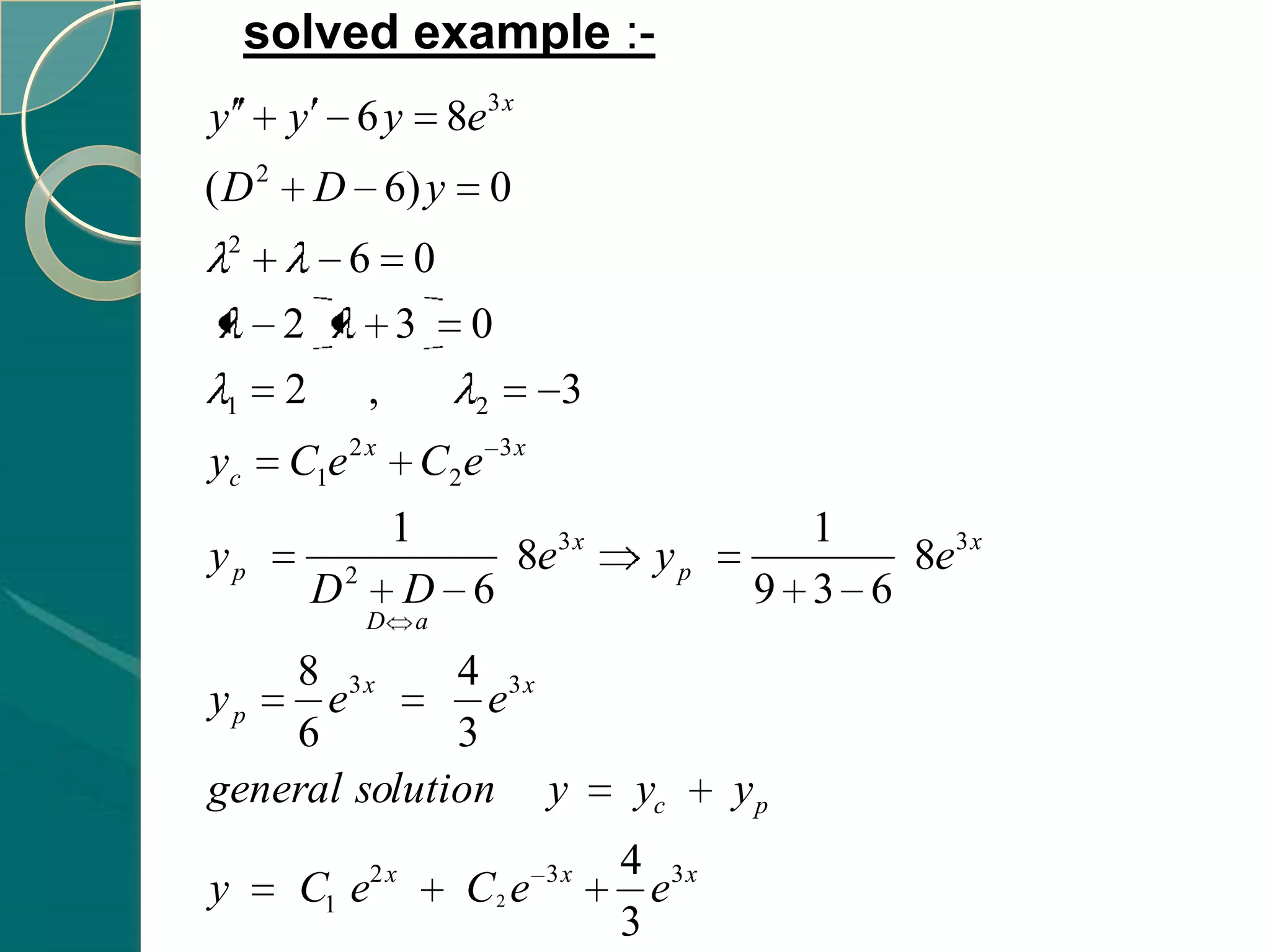
L(D) y = f (x) non-homogeneous
the general solution of non-homogeneous is
y = yc + yp
yc complement solution
[solution of homogeneous equation L(D) y = 0 look last slide]
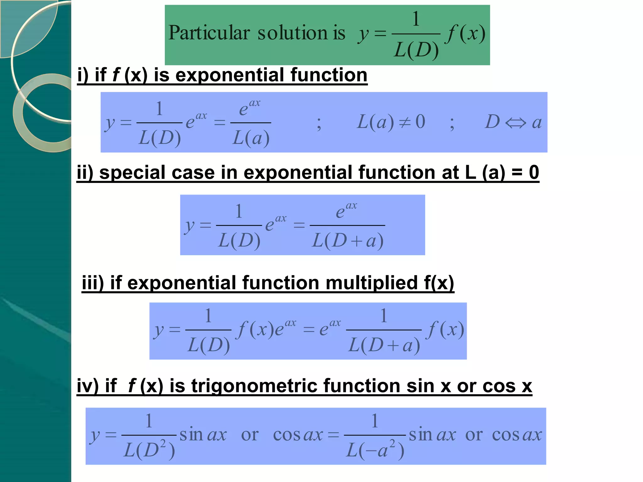
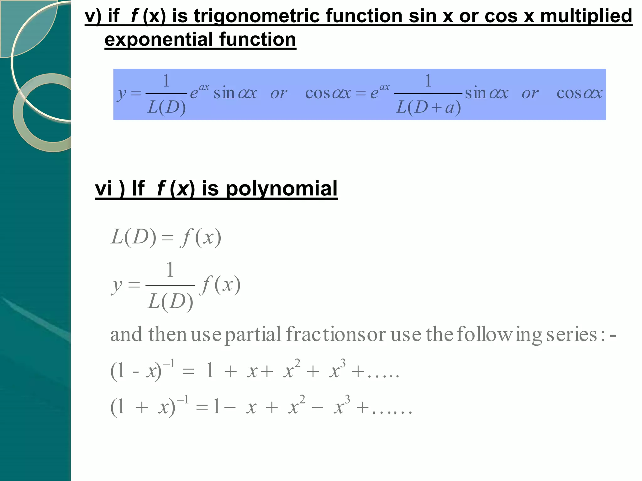
y p particular solution is Note
L(D) is differential
1 effective
y f ( x) 1 / L(D) is integral
L( D) effective
We knew how to get the complement
solution last slide. To get the particular solution it depends on the type
of function we will know the different types and example to every
one as following .](https://image.slidesharecdn.com/ordinarydifferentialequations-130408184155-phpapp02/75/Ordinary-differential-equations-29-2048.jpg)


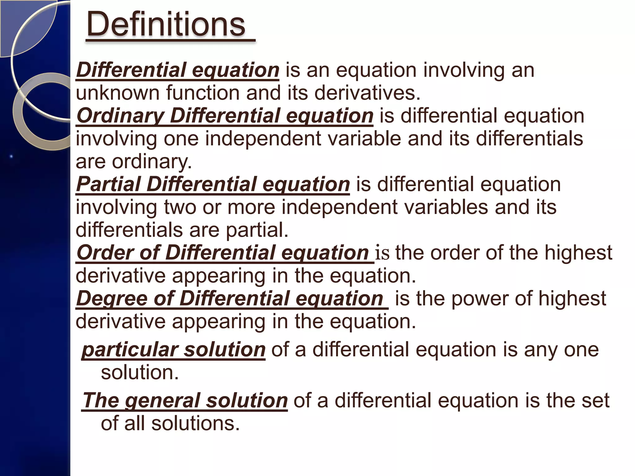
The document is an introduction to ordinary differential equations prepared by Ahmed Haider Ahmed. It defines key terms like differential equation, ordinary differential equation, partial differential equation, order, degree, and particular and general solutions. It then provides methods for solving various types of first order differential equations, including separable, homogeneous, exact, linear, and Bernoulli equations. Specific examples are given to illustrate each method.