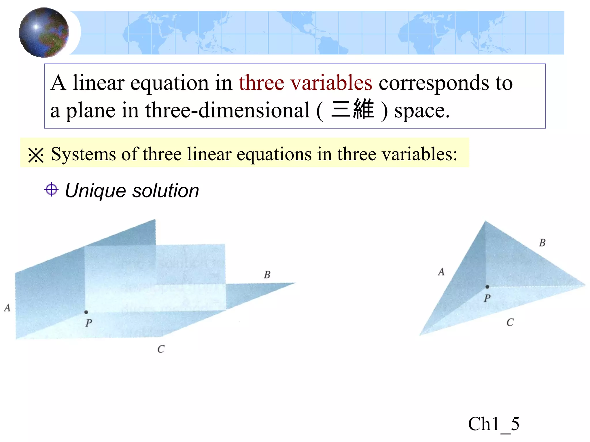
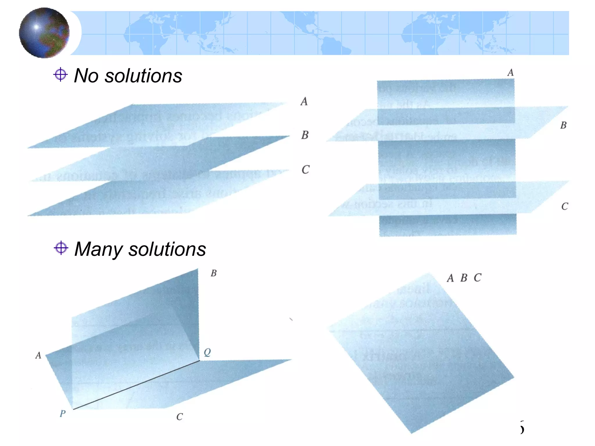
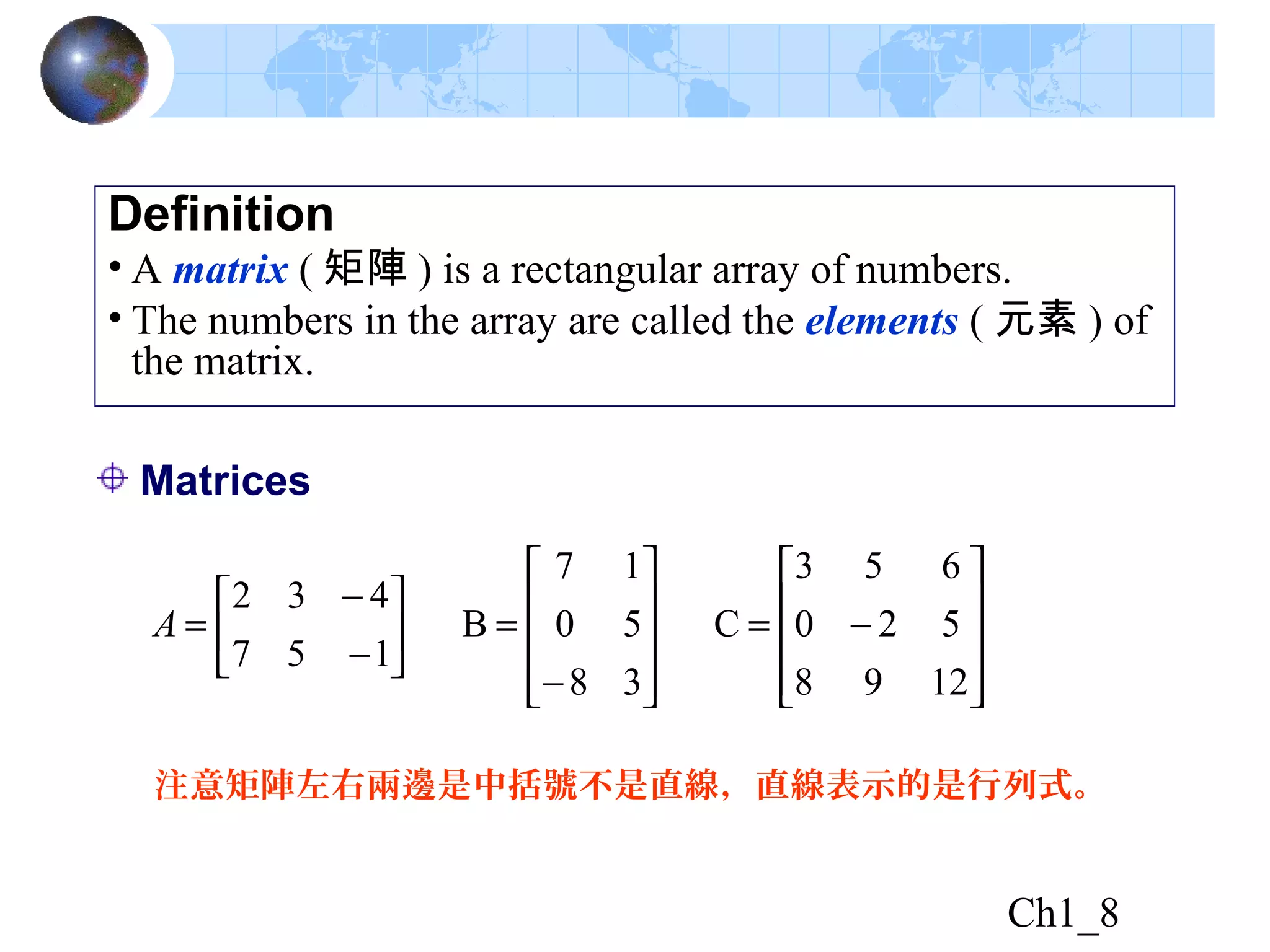
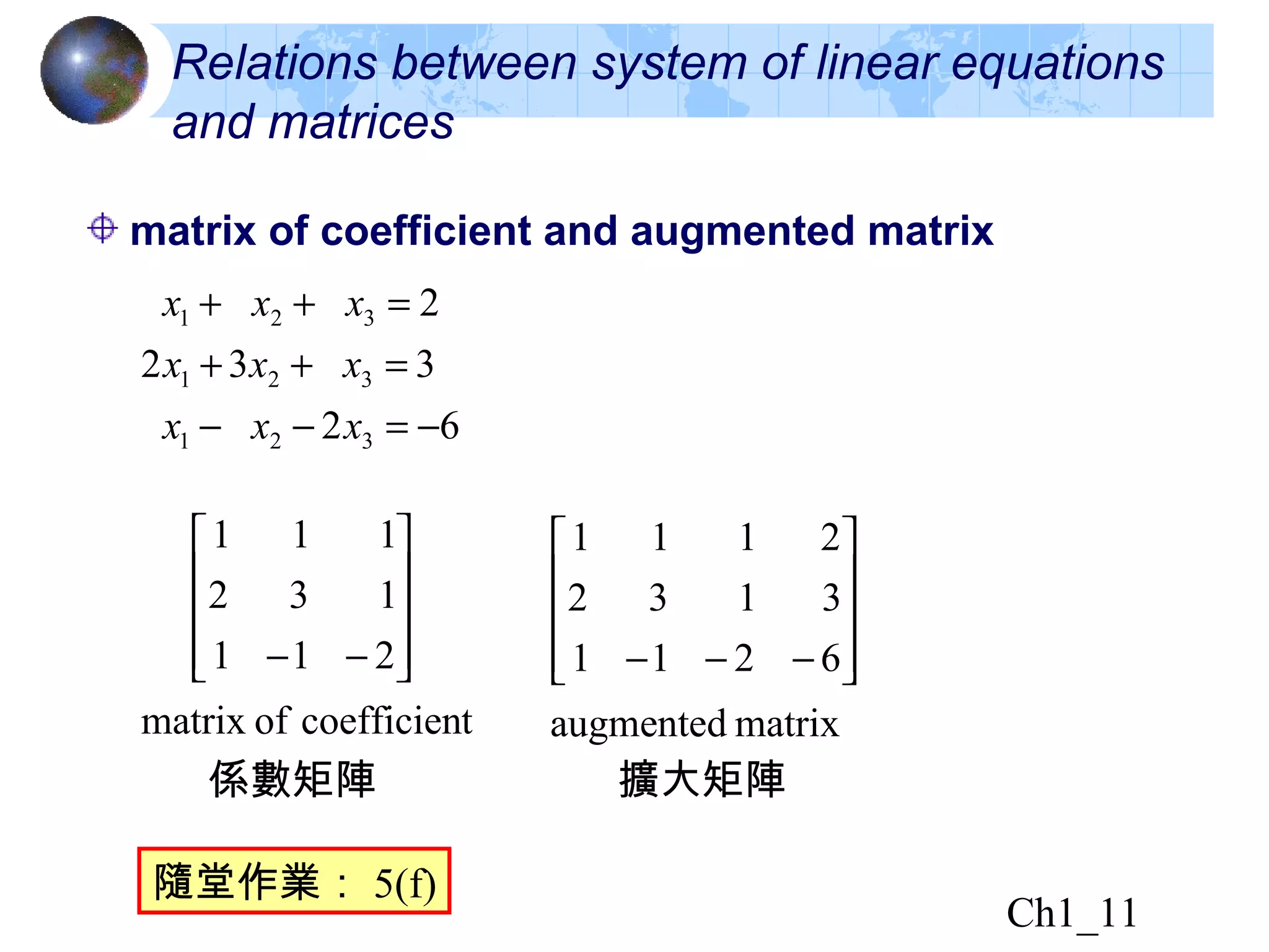
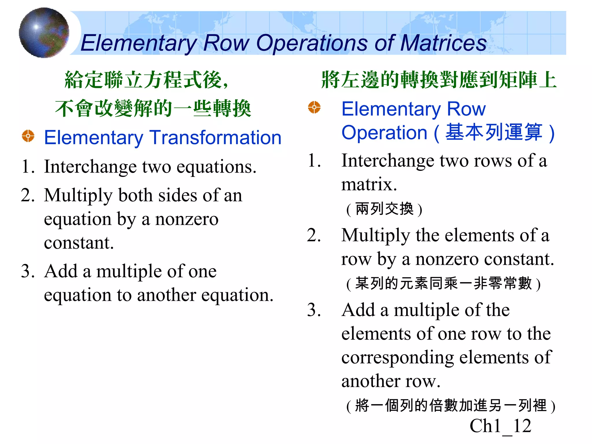
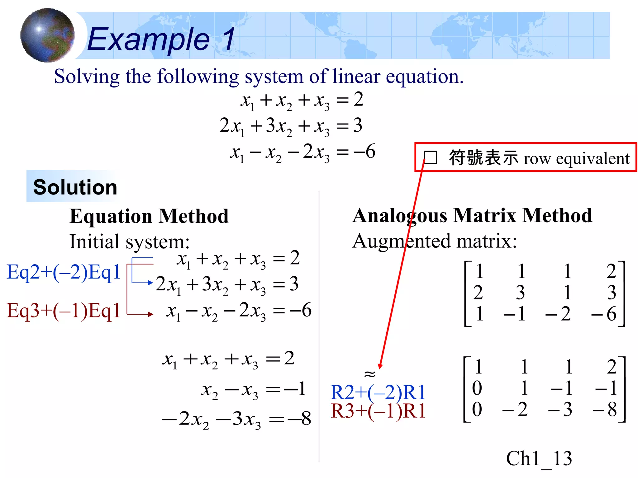
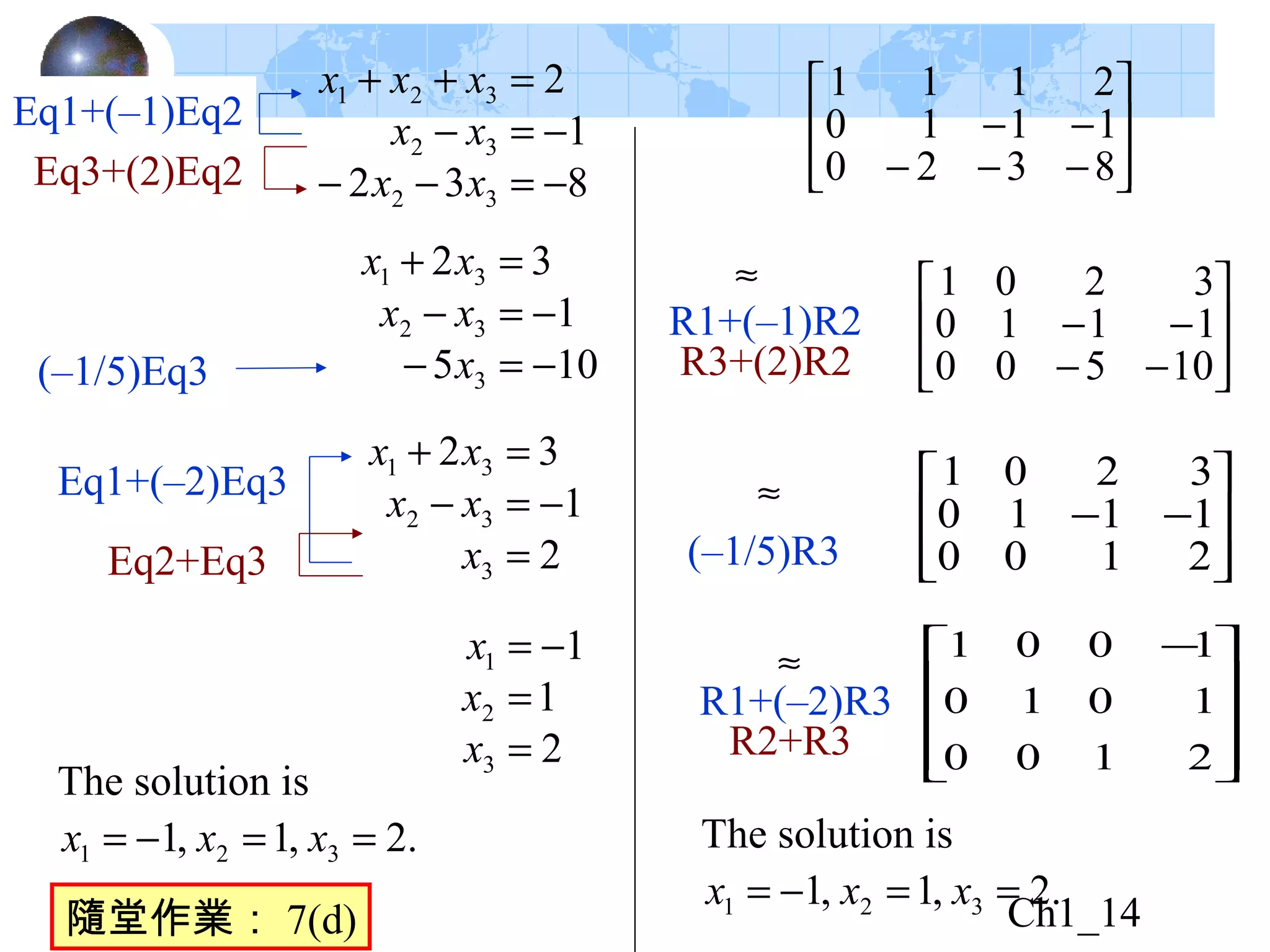
This document introduces systems of linear equations and matrix operations. It defines linear equations, solutions, and graphs related to systems of linear equations. It also defines matrices, matrix operations, and the relationship between systems of linear equations and matrices. Specifically, it describes how a system of linear equations can be represented by an augmented matrix and how elementary row operations on a matrix correspond to elementary transformations of the associated system of linear equations.
![Ch1_9
Submatrix ( 子矩陣 )
Amatrix
215
032
471
−
=A
Row ( 列 ) and Column ( 行 )
[ ] [ ]
3column2column1column2row1row
1
4
5
3
7
2
157432
−
−
−−
157
432
−
−
=A
Aofssubmatrice
25
41
1
3
7
15
32
71
−
=
=
= RQP](https://image.slidesharecdn.com/linearalgebra-131010034008-phpapp02/75/Linear-algebra-9-2048.jpg)
![Ch1_10
Identity Matrices ( 單位矩陣 )
diagonal ( 對角線 ) 上都是 1 ,其餘都是 0 , I 的下標表示 size
=
=
100
010
001
10
01
32 II
Location
7,4
157
432
2113 =−=
−
−
= aaA
aij 表示在 row i, column j 的元素值
也寫成 location (1,3) = −4
Size and Type
[ ]
matrixcolumnamatrixrowamatrixsquarea
matrix13matrix41matrix3332:Size
2
3
8
5834
853
109
752
542
301
××××
−
−
−
−](https://image.slidesharecdn.com/linearalgebra-131010034008-phpapp02/75/Linear-algebra-10-2048.jpg)
![Ch1_17
Summary
−−−
−
−
=
7012
32863
441284
]:[ BA
A BUse row operations to [A: B] :
.
1100
3010
2001
−
≈≈
−−−
−
−
7012
32863
441284
]:[]:[ XIBA n≈≈i.e.,
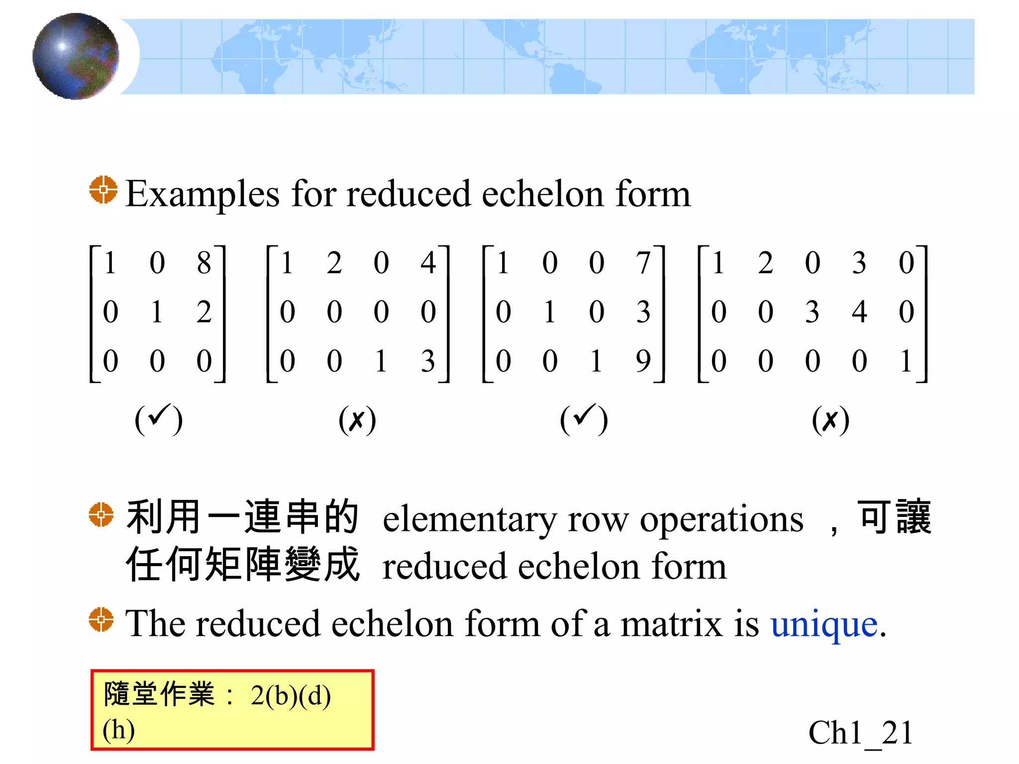
Def. [In : X] is called the reduced echelon form ( 簡化梯
式 )
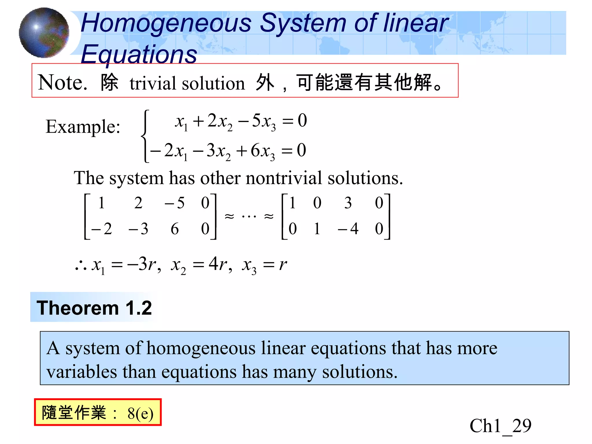
of [A : B].Note. 1. If A is the matrix of coefficients of a system of n equations
in n variables that has a unique solution,
then A is row equivalent to In (A ≈ In).
2. If A ≈ In, then the system has unique solution.
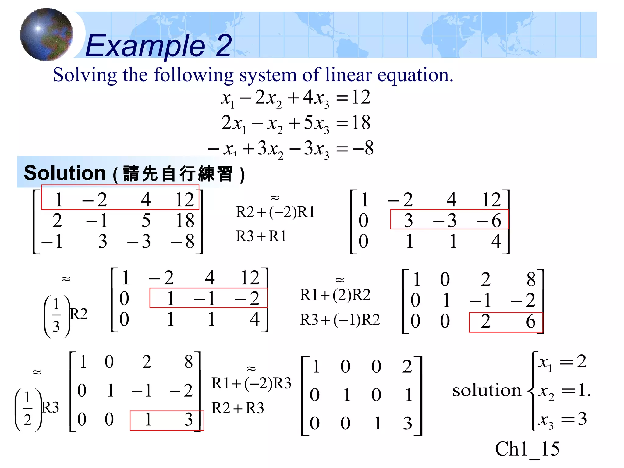
72
32863
441284
21
321
321
−=−−
=−+
=−+
xx
xxx
xxx](https://image.slidesharecdn.com/linearalgebra-131010034008-phpapp02/75/Linear-algebra-17-2048.jpg)


![3.6 systems and matrices[1]](https://cdn.slidesharecdn.com/ss_thumbnails/3-6systemsandmatrices1-121025102540-phpapp02-thumbnail.jpg?width=640&height=640&fit=bounds)


![Vibe Coding vs. Spec-Driven Development [Free Meetup]](https://cdn.slidesharecdn.com/ss_thumbnails/vibecodingvsspecdrivendevelopment-251209105622-43f455e7-thumbnail.jpg?width=640&height=640&fit=bounds)


