This document details how to extract risk severity information from the standard risk matrix.

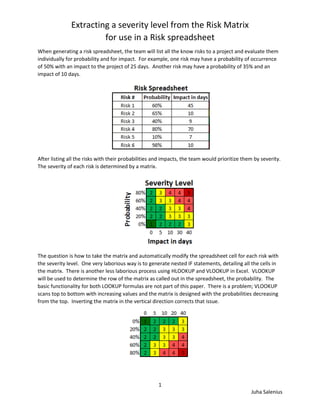
1. Extracting a severity level from the Risk Matrix
for use in a Risk spreadsheet
When generating a risk spreadsheet, the team will list all the know risks to a project and evaluate them
individually for probability and for impact. For example, one risk may have a probability of occurrence
of 50% with an impact to the project of 25 days. Another risk may have a probability of 35% and an
impact of 10 days.
After listing all the risks with their probabilities and impacts, the team would prioritize them by severity.
The severity of each risk is determined by a matrix.
The question is how to take the matrix and automatically modify the spreadsheet cell for each risk with
the severity level. One very laborious way is to generate nested IF statements, detailing all the cells in
the matrix. There is another less laborious process using HLOOKUP and VLOOKUP in Excel. VLOOKUP
will be used to determine the row of the matrix as called out in the spreadsheet, the probability. The
basic functionality for both LOOKUP formulas are not part of this paper. There is a problem; VLOOKUP
scans top to bottom with increasing values and the matrix is designed with the probabilities decreasing
from the top. Inverting the matrix in the vertical direction corrects that issue.
1
Juha Salenius

2. Extracting a severity level from the Risk Matrix
for use in a Risk spreadsheet
Now VLOOKUP will work correctly. The next step is to find the correct column. HLOOKUP is used for
that but there is a problem. If we nest the HLOOKUP within the VLOOKUP, VLOOKUP is requiring a
column number not a duration. Adding an additional row to the matrix starting from the left side and
counting up to 6, in this example, will provide the correct column number for the VLOOKUP formula.
VLOOKUP(Probability, v matrix,(HLOOKUP(impact in days, h matrix,last row,not exact)),not exact)
Shown below is the completed matrix with a small portion of a risk spreadsheet.
In the matrix above, the red rectangle is the V matrix, the green rectangle is the H matrix. Notice the
HLOOKUP values at the bottom of the matrix in row 7. Those numbers provide the result for the
HLOOKUP formula. The Blue and purple cell selected in the risk spreadsheet are the probability used in
the VLOOKUP and the Impact in days used in the HLOOKUP formulas respectively. The result cell is
highlighted showing the formula contained in the cell in the formula bar above.
The cells can then befilled with the correct color for the value returned using conditional formatting.
Making the risk level number the same color as the fill color eliminates clutter. But the number for the
risk severity level is embedded within the conditional formatting of the Result cells so the user can sort
the spreadsheet to determine the high priority risks for further work; mitigation and contingency
planning.
EOF
2
Juha Salenius