This document provides a step-by-step tutorial for creating a sales funnel chart in Excel. It begins by outlining some of the problems with funnel charts, such as how they can mislead readers by not proportionally representing data. It then explains that executives still want to see these charts despite the issues. The tutorial shows how to take a stacked pyramid chart and modify it through flattening, flipping, and labeling to resemble a funnel. The 7 steps include selecting the chart type, switching rows and columns, adjusting rotation, reversing the axis order, cleaning up labels and grids, and adding data labels.

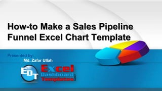
1. Presented by:
Md. Zafar Ullah
How-to Make a Sales Pipeline
Funnel Excel Chart Template

2. HEAD or TAIL
- Problems with Funnel chart
- Then Why?
6/18/2013 2

3. Problems with Funnel Chart
• The chart may have the potential to mislead
readers.
• The area of each section may not represent the
data proportionally to other sections.
– For instance, if your values for each section/category are
the same, then the size of the top section is not
proportionally equal to the bottom section even though
they are the same value.
6/18/2013 3

4. • So be careful when using this as a
representation of your data.
6/18/2013 4
• In this graphic, it can be deceiving to
readers that the Sales in Prospecting
phase are much larger than those in
the Negotiation phase, when in
reality, they are exactly equal.
• The graphic is basing the height on
the category value, not the width or
volume of the section.
Problems with Funnel Chart (cont.)

5. Then Why?
• Even though this may be a bad graphic from
all design and data visualization perspectives,
you may be asked to create this type of
graphic for your Executive Dashboard.
– Your first step should be to talk with the powers that be
about the issues with this type of chart.
– If your client or executives or managers still want this as
pare of the Company Dashboard, then give the people what
they want.
– That is why you will see this type of chart in many well-
known software packages like Salesforce.com.
6/18/2013 5

6. 6/18/2013 6
• Lets say you are the
Dashboard Designer for your
sales organization.
Then Why? (cont.)

7. • Lets say that your sample data
has categories from your sales
organization on how the sales
pipeline looks for the
company.
6/18/2013 7
• This is your data in Excel.
– Presently there are 652 sales opportunities in the Prospecting stage
worth $33.6M.
– This is the start of the sales cycle for your company and each sales
opportunity may be at a different level in the sales cycle.
Then Why? (cont.)

8. 6/18/2013 8
- Typically there are less and less
at each progressive stage of the
sales cycle because deals are not
always a done deal.
- Some people in the prospecting
stage may change their mind
and not purchase anything.
- Another potential sale that is in the Presentation stage may not get
closed because the buyer chose another company to handle the
business.
Exceldatafile Then Why? (cont.)

9. 6/18/2013 9
- However, not all sales fall out of
the pipeline and your
organization may be able to
calculate the likely percentage
that any given opportunity may
close from each stage of the
sales cycle.
- This is why organizations like to see this data in a pipeline or
funnel format because each stage fills the next stage in the cycle.
- And if you don’t have enough sales in each part of the pipeline,
your company will have uneven cash flows as each sale will most
likely have an average closing time from start to finish.
Exceldatafile Then Why? (cont.)

10. HOW TO MAKE FUNNEL
CHART in EXCEL
- Sales Funnel or Sales Pipeline Chart or Graph in Excel
- The Breakdown
- Step-by-Step Tutorial
6/18/2013 10

11. Funnel Chart or Graph in Excel
6/18/2013 11

12. Funnel Chart or Graph in Excel
- Looking at the standard set of charts
that are available in Excel, the closest
representation of what we are looking
for is a Stacked Pyramid chart.
- More specifically, a 100% Stacked
Pyramid chart since our data
represents 100% of the sales pipeline
data and we are not trying to compare
the data from one pyramid to another.
- You will find the 100% Stacked
Pyramid chart under the Column
Chart menu in the Insert Ribbon.
6/18/2013 12

13. The Breakdown
6/18/2013 13
1) Create a 100% Stacked Pyramid Chart
2) Flatten it to 2D
3) Flip it upside down
4) Label and Clean it up

14. Step-by-Step Tutorial
6/18/2013 14
1) Highlight the Data from
A2:B6 (From “Prospecting” to
Negotiation Value of “45”) and from
the Insert Ribbon, choose the Column
Menu from the Charts Group and then
select 100% Stacked Pyramid.

15. Step-by-Step Tutorial (cont.)
6/18/2013 15
The resulting chart will look like above

16. 6/18/2013 16
2) In the chart, select the
data series for Series one by
clicking on the
pyramids. Then from the
“Design Ribbon”, select
“Switch Row/Column” from
the Data Group.
Step-by-Step Tutorial (cont.)

17. Step-by-Step Tutorial (cont.)
6/18/2013 17
The resulting chart will look like above

18. Step-by-Step Tutorial (cont.)
6/18/2013 18
The resulting chart will look like above
The funnel chart is
starting to take shape.

19. 6/18/2013 19
3) Right click on the chart and
select “3D Rotation…” from
the menu or you can also see
this as a choice from the
Layout Ribbon in the
Background Group.
Step-by-Step Tutorial (cont.)

20. 6/18/2013 20
4) Change the Rotation
Settings as follows:
X=0
Step-by-Step Tutorial (cont.)

21. 6/18/2013 21
4) Change the Rotation
Settings as follows:
Y=0
Step-by-Step Tutorial (cont.)

22. 6/18/2013 22
4) Change the Rotation
Settings as follows:
Y=0
Step-by-Step Tutorial (cont.)
Now we are getting really close to the Final
Sales Funnel Chart in Excel.

23. 6/18/2013 23
5) Right click on the chart’s
Vertical Axis and select
“Format Axis…” from the
menu or you can also see
this as the Primary Vertical
Axis choice from the Layout
Ribbon in the Axis Group.
Step-by-Step Tutorial (cont.)

24. 6/18/2013 24
5) and choose “Values in
reverse order” from the Axis
Options Dialog Box.
Step-by-Step Tutorial (cont.)

25. 6/18/2013 25
5) and choose “Values in
reverse order” from the Axis
Options Dialog Box.
Step-by-Step Tutorial (cont.)
Now we just need to clean up the Chart and
give it some Data Labels.

26. 6/18/2013 26
• Remove the Vertical Axis – Click on the Vertical
Axis and press your delete key.
• Remove the Legend – Click on the Legend and
press your delete key.
• Remove the Horizontal Gridlines – Click on the
horizontal Gridlines and press your delete key.
• Remove the Category Label – Click on the #1 at
the top of the Sales Funnel and press your delete
key.
• Add Data Labels – Click anywhere in the chart and
change Data Labels to “Show” from the Layout
Ribbon in the Labels Group.
6) Clean
up
Step-by-Step Tutorial (cont.)

27. 6/18/2013 27
7) Admire your handy work.
Step-by-Step Tutorial (cont.)
Your Sales Funnel for Excel should now be
completed and should look like this.

29. Thanks for viewing this presentation
Please remember to sign up for the RSS Feed and
also leave a comment on the other types of charts
you would like to see.
6/18/2013 29