![D. Shukla, Rahul Singhai, Surendra Gadewar, Saurabh jain, Shewta Ojha, P.P. Mishra
International Journal of Computer Networks (IJCN), Volume (2): Issue (2) 141
1. REVIEW OF LITERATURE
Ko and Davis [3] proposed a protocol known as space-division multiple access (SDMA) which is
useful for a satellite switched communication network. Abott [1] discussed a new technique for
switching system using digital Space-Division concept for dealing with high-speed data signals.
Yamada et al. [16] derived the high-speed digital switching technology with the help of space-
division switches. Karol et al. [8] presented an input versus output analysis of queuing on a
space-division packet switching. In a contribution Li [5] performed analysis for non-uniform traffic
in the setup of Space-Division switches. Yamanka et al. [17] expanded space-division (SD) switch
architecture and suggested a bipolar circuit design for gigabit-per-second cross-point switch LSIs.
Lee and Li [4] have studied the performance of a non blocking space-division packet switch using
finite-state Markov chain model, given the traffic intensities changes as a function of time. Li [6]
derived the performance of a non blocking space-division packet switch in a correlated input
traffic environment. Wang and Tobagi [14] suggested a self-routing space-division fast packet
switch architecture achieving output queuing with a reduced number of internal path. Cao [2]
derived a discrete-time queuing network model for space-division packet switches. Pao and
Leung [10] used space-division approach to implement a shared buffer in an ATM switch which
does not require scaling up the bandwidth of the shared memory. Shukla, Singhai & Gadewar
[12] presented Markov Chain analysis for reaching probabilities of message flow in space division
switches.
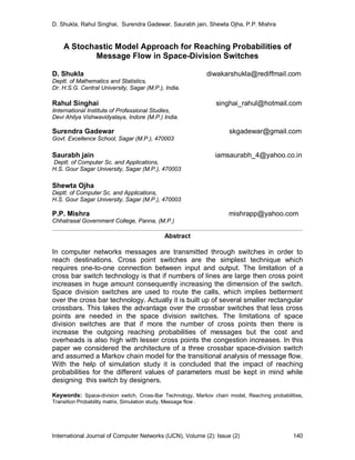
FIGURE 1: Three cross bar space division switch
2. MOTIVATION
Shukla and Gadewar [11] have suggested a Markov chain model for the transitional analysis of
message flow in a two crossbar space division switches. We extend this model, in this paper,
Crossbars
n
N
Crossbars
n
N
Crossbarst
K
M
L
L
L
L
a1
a2
n
N
n
N
b1
b2
b3
tn
tn
tn
tn
d1
c1
f1e1
g1 h1
n
N
n
N
n
N
n
N
n
N
n
N
i1
j1
nt
nt
nt
nt loss
loss
loss
loss](data:image/gif;base64,R0lGODlhAQABAIAAAAAAAP///yH5BAEAAAAALAAAAAABAAEAAAIBRAA7)
Recommended
Recommended
More Related Content
Similar to A Stochastic Model Approach for Reaching Probabilities of Message Flow in Space-Division Switches
Similar to A Stochastic Model Approach for Reaching Probabilities of Message Flow in Space-Division Switches (20)
Recently uploaded
Recently uploaded (20)
A Stochastic Model Approach for Reaching Probabilities of Message Flow in Space-Division Switches
- 1. D. Shukla, Rahul Singhai, Surendra Gadewar, Saurabh jain, Shewta Ojha, P.P. Mishra International Journal of Computer Networks (IJCN), Volume (2): Issue (2) 140 A Stochastic Model Approach for Reaching Probabilities of Message Flow in Space-Division Switches D. Shukla diwakarshukla@rediffmail.com Deptt. of Mathematics and Statistics, Dr. H.S.G. Central University, Sagar (M.P.), India. Rahul Singhai singhai_rahul@hotmail.com Iinternational Institute of Professional Studies, Devi Ahilya Vishwavidyalaya, Indore (M.P.) India. Surendra Gadewar skgadewar@gmail.com Govt. Excellence School, Sagar (M.P.), 470003 Saurabh jain iamsaurabh_4@yahoo.co.in Deptt. of Computer Sc. and Applications, H.S. Gour Sagar University, Sagar (M.P.), 470003 Shewta Ojha Deptt. of Computer Sc. and Applications, H.S. Gour Sagar University, Sagar (M.P.), 470003 P.P. Mishra mishrapp@yahoo.com Chhatrasal Government College, Panna, (M.P.) Abstract In computer networks messages are transmitted through switches in order to reach destinations. Cross point switches are the simplest technique which requires one-to-one connection between input and output. The limitation of a cross bar switch technology is that if numbers of lines are large then cross point increases in huge amount consequently increasing the dimension of the switch. Space division switches are used to route the calls, which implies betterment over the cross bar technology. Actually it is built up of several smaller rectangular crossbars. This takes the advantage over the crossbar switches that less cross points are needed in the space division switches. The limitations of space division switches are that if more the number of cross points then there is increase the outgoing reaching probabilities of messages but the cost and overheads is also high with lesser cross points the congestion increases. In this paper we considered the architecture of a three crossbar space-division switch and assumed a Markov chain model for the transitional analysis of message flow. With the help of simulation study it is concluded that the impact of reaching probabilities for the different values of parameters must be kept in mind while designing this switch by designers. Keywords: Space-division switch, Cross-Bar Technology, Markov chain model, Reaching probabilities, Transition Probability matrix, Simulation study, Message flow .
- 2. D. Shukla, Rahul Singhai, Surendra Gadewar, Saurabh jain, Shewta Ojha, P.P. Mishra International Journal of Computer Networks (IJCN), Volume (2): Issue (2) 141 1. REVIEW OF LITERATURE Ko and Davis [3] proposed a protocol known as space-division multiple access (SDMA) which is useful for a satellite switched communication network. Abott [1] discussed a new technique for switching system using digital Space-Division concept for dealing with high-speed data signals. Yamada et al. [16] derived the high-speed digital switching technology with the help of space- division switches. Karol et al. [8] presented an input versus output analysis of queuing on a space-division packet switching. In a contribution Li [5] performed analysis for non-uniform traffic in the setup of Space-Division switches. Yamanka et al. [17] expanded space-division (SD) switch architecture and suggested a bipolar circuit design for gigabit-per-second cross-point switch LSIs. Lee and Li [4] have studied the performance of a non blocking space-division packet switch using finite-state Markov chain model, given the traffic intensities changes as a function of time. Li [6] derived the performance of a non blocking space-division packet switch in a correlated input traffic environment. Wang and Tobagi [14] suggested a self-routing space-division fast packet switch architecture achieving output queuing with a reduced number of internal path. Cao [2] derived a discrete-time queuing network model for space-division packet switches. Pao and Leung [10] used space-division approach to implement a shared buffer in an ATM switch which does not require scaling up the bandwidth of the shared memory. Shukla, Singhai & Gadewar [12] presented Markov Chain analysis for reaching probabilities of message flow in space division switches. FIGURE 1: Three cross bar space division switch 2. MOTIVATION Shukla and Gadewar [11] have suggested a Markov chain model for the transitional analysis of message flow in a two crossbar space division switches. We extend this model, in this paper, Crossbars n N Crossbars n N Crossbarst K M L L L L a1 a2 n N n N b1 b2 b3 tn tn tn tn d1 c1 f1e1 g1 h1 n N n N n N n N n N n N i1 j1 nt nt nt nt loss loss loss loss
- 3. D. Shukla, Rahul Singhai, Surendra Gadewar, Saurabh jain, Shewta Ojha, P.P. Mishra International Journal of Computer Networks (IJCN), Volume (2): Issue (2) 142 from two-crossbars to three crossbar setup and with the help of a simulation study, the impact on reaching probabilities of message is analyzed. 3. INTRODUCTION AND ASSUMPTIONS In what follows, we consider a space-division switch [11],[12] with parameters 3,4,16 tnN shown in fig. 1 and assume the followings: a) The left side of switches is input and the flow of information is from left to right. b) Each input line, on left side, is attached with a computer having different initial probabilities of selection by users. This level is the stage 1. c) The middle crossbars are stage 2 containing three crossbars with each having four inputs and four output lines. d) The third stage contains four crossbars, each with three inputs and four output lines. At this, three output lines are with computers and the fourth one, in each crossbar, is a loss state. e) The term I(M,K,L) denotes an input state at Mth stage in Kth crossbar and at Lth input line where M=1,2,3;K=1,2,3,4;L=1,2,3,4. For example, in fig. 1 the term 1a is input state I(1,1,1), a2 is state I(1,1,2), c1 is I(1,2,1),e1 is I(2,1,1), g1 is I(2,2,1), and i1 is I(3,1,1). f) The term O(M,K,L) denotes output state at M th stage, in K th crossbar and L th output line like the term b1 is output state O(1,1,1), b2 is O(1,1,2), b3 is O(1,1,3), d1 is O(1,2,1), f1 is O(2,1,1), h1 is O(2,2,1) and j1 is O(3,1,1). As special, the output states O(3,1,4), O(3,2,4), O(3,3,4) and O(3,4,4) are loss states and when a message reaches to them, it is assumed lost or reached to the known destinations. 3.1. Markov Chain Model Let {Xn , n = 0,1,2,3….} be a Markov chain with state space I(M,K,L) and O(M,K,L), M=1,2,3 and K,L = 1,2,3,4. The Xn denotes the state of message at the nth step transition over states I(M,K,L) and O(M,K,L). The unit-step transition probabilities over states are: )(1,,13,,1 ,,12,,1 ,,11,,1 211 21 11 kKnn Knn Knn LLLKIXKOXP LLKIXKOXP LLKIXKOXP When L=1,2,3;K=1,2,3,4 3,2,1 ,,,1,,11 Jwhen PJKOXLKIXP LKnn JKOXLKIXP nn ,,1,,11 3,2,11,2,3,4;;41 3 1 JKLwhenP i iK LKOXLKIXP LKIXLKOXP nn nn ,,2,,2 ,,2,,2 12 12 1,2,31,2,3;, KLwhenQLK 1,2,3,;4 ,1),,2(/),,2( ,,2,,2 3 1 12 12 KLwhen QLkOXLkIXP LKIXLKOXP i iKnn nn LKOXLKIXP LKIXLKOXP nn nn ,,2,,2 ,,2,,2 12 12
- 4. D. Shukla, Rahul Singhai, Surendra Gadewar, Saurabh jain, Shewta Ojha, P.P. Mishra International Journal of Computer Networks (IJCN), Volume (2): Issue (2) 143 1,21,2,3;, KLwhenQLK 3,2,11,2,3,4;;3,2,1 ,,,3,,3 23 JKLwhen RJKIXLKOXP LKnn 3,2,11,2,3,4;;4,1 ,,34,,3 3 1 23 JKLwhenR JKIXKOXP i iK nn 4,3,2,1;3,2,1 1,,33,,3 ,,32,,3 ,,31,,3 2 1 23 223 123 KLwhen SLKOXKIXP SLKOXKIXP SLKOXKIXP i iKnn Knn Knn The terms LiK, SiK ,PiK, QiK ,RiK (i=1,2,3) are the probabilities of transition lying between 0 and 1 and placed as elements of transition probability matrix given below. 1,,1 KI 2,,1 K 3,,1 KI 4,,1 KI 1,,1 KO 2,,1 KO 3,,1 KO 1,,1 KI 0 0 0 0 L1k L2k )kLk(1 21 L 2,,1 KI 0 0 0 0 L1k L2k )kLk(1 21 L 3,,1 KI 0 0 0 0 L1k L2k )kLk(1 21 L 4,,1 KI 0 0 0 0 L1k L2k )kLk(1 21 L 1,,1 KO P1k P2k P3k )kPkP kP(1 32 1 0 0 0 2,,1 KO P1k P2k P3k )kPkPkP(1 321 0 0 0 3,,1 KO P1k P2k P3k )kPkPkP(1 321 0 0 0 TABLE 1: Transition probability matrix (t. p. m.) for stage 1 1,,1 KI 2,,1 K 3,,1 KI 4,,1 KI 1,,1 KO 2,,1 KO 3,,1 KO 1,,1 KI 0 0 0 0 L1k L2k )kLk(1 21 L 2,,1 KI 0 0 0 0 L1k L2k )kLk(1 21 L 3,,1 KI 0 0 0 0 L1k L2k )kLk(1 21 L 4,,1 KI 0 0 0 0 L1k L2k )kLk(1 21 L 1,,1 KO P1k P2k P3k )kPkP kP(1 32 1 0 0 0 2,,1 KO P1k P2k P3k )kPkPkP(1 321 0 0 0 3,,1 KO P1k P2k P3k )kPkPkP(1 321 0 0 0 TABLE 2: Transition probability matrix (t. p. m.) for stage 2 States States e States States e
- 5. D. Shukla, Rahul Singhai, Surendra Gadewar, Saurabh jain, Shewta Ojha, P.P. Mishra International Journal of Computer Networks (IJCN), Volume (2): Issue (2) 144 1,,3 KI 2,,3 KI 3,,3 KI 1,,3 KO 2,,3 KO 3,,3 KO 4,,3 KO 1,,3 KI 0 0 0 R1k R2k R3k )kRkRkR(1 321 2,,3 KI 0 0 0 R1k R2k R3k )kRkRkR(1 321 3,,3 KI 0 0 0 R1k R2k R3k )kRkRkR(1 321 1,,3 KO S1k S2k )kSkS(1 21 0 0 0 0 2,,3 KO S1k S2k )kSkS(1 21 0 0 0 0 3,,3 KO S1k S2k )kSkS(1 21 0 0 0 0 4,,3 KO S1k S2k )kSkS(1 21 0 0 0 0 TABLE 3: Transition probability matrix (t. p. m.) for stage 3 3.2. Model Classification The probabilities Li k , Pi k , Q i k , R i k and Si k may be functions of M, K and L parameters and on this basis the classification of Markov chain models be as below: M-Dependent model- where probabilities Li k , Pi k , Q i k , R i k and Si k are only functions of M. K-Dependent model- where probabilities Li k , Pi k , Q i k , R i k and Si k are only functions of K L-Dependent model- where probabilities are functions of K and L parameters both. 4. CALCULATION OF REACHING (INITIAL) PROBABILITIES Let Pik ( I = 1,2,3 ) be the probability of choosing the ith input line in Kth switching element of the space division switch configuration given in fig. 1of the section 1.0. For 4i , the probability is 3 1 1 i iKp . For the Markov chain {Xn , n = 0,1,2,3….} over the states I(M,K,L), the initial probabilities of choosing a connecting path is KpKIXP 10 1,,1 , K pKIXP 20 2,,1 KpKIXP 30 3,,1 , kkkK ppppKIXP 32140 14,,1 3 1 1 i iK p 4.1. Outgoing Probabilities At Stage 1, 2 and 3 The O(1,K,L) over varying K and L are the outgoing states, for the stage 1, where the message is ready to route into for the next stage. P [ X 1 = O(1,K,L) ] =P[ message reaches to the state O(1,K,L) at the first step] The general form for M = 1(stage-1) is P [x = O (1, k, L)] = L1 k when L = 1;K = 1, 2, 3, 4 States e States
- 6. D. Shukla, Rahul Singhai, Surendra Gadewar, Saurabh jain, Shewta Ojha, P.P. Mishra International Journal of Computer Networks (IJCN), Volume (2): Issue (2) 145 = L1`k when L = 2 = {1 – L1 k + L2 k } when L = 3 The general form for M = 2 (stage-2) is P [x = O (2, k, L)] = QLK 4 1 1 i iL when k = 1, L = 1, 2,3 P [x=O(2,k,L)] = {1- 3 1i ikQ } 4 1 1 i i L when k = 1, L = 4 P [x= O (2, k, L)] = QLK 4 1 2 i i L when k = 2,L = 1, 2,3 P [x= O(2,k,L)] ={1- 3 1i ikQ } 4 1 2 i i L when k = 2,L= 4 P[x=O(2,k,L)]=QLK{4- 4 1 1 i iL - 4 1 2 i iL } when k=3, L= 1,2,3 P [x = O (2, k, L)] = {1- 3 1i ikQ } {4 - 4 1 1 i iL - 4 1 2 i i L } when k = 3, L = 4 The general form for m = 3(stage-3) is P [x = O (3, k, L)] = R LK * 4 1 2 4 1 13 4 1 22 4 1 11 4 i i i ik i ik i ik LLQLQLQ when k = 1, 2, 3 ; L = 1, 2, 3 P[x=O(3,k, L)] = R LK * *1 3 1 i ik R 4 1 2 4 1 13 4 1 22 4 1 11 4 i i i ik i ik i ik LLQLQLQ when k = 1, 2, 3 , L = 4 P[x=O(3,k,L)] =RLK 4 1 2 4 1 1 3 1 3 4 1 2 3 1 2 4 1 1 3 1 1 41 11 i i i i i i i i i i i i i i LLQ LQLQ when K = 4 , L = 1, 2, 3 P[x=O(3,k,L)]= 3 1 1 i ik R * 4 1 2 4 1 1 3 1 3 4 1 2 3 1 2 4 1 1 3 1 1 41 11 i i i i i i i i i i i i i i LLQ LQLQ when k = 4 , L = 4 5. K-Dependent Model and Simulation Study Consider the following K-dependent Markov chain model with unit-step transition probabilities 4,3,2,1 321,,1,,1 2,1,,1,,1 01 01 L JwhenaKLKIXJKOXP JwhenaKLKIXJKOXP K K
- 7. D. Shukla, Rahul Singhai, Surendra Gadewar, Saurabh jain, Shewta Ojha, P.P. Mishra International Journal of Computer Networks (IJCN), Volume (2): Issue (2) 146 3,2,1 431,,1,,1 3,2,1,,1,,1 01 01 L JwhenbKLKOXJKIXP JwhenbKLKOXJKIXP K K 4,3,2,1 431,,2,,2 3,2,1,,2,,2 12 12 L JwhencKLKIXJKOXP JwhencKLKIXJKOXP K K 4,3,2,1 431,,2,,2 3,2,1,,2,,2 12 12 L JwhencKLKOXJKIXP JwhencKLKOXJKIXP K K 3,2,1 431,,3,,3 3,2,1,,3,,3 23 23 L JwhendKLKIXJKOXP JwhendKLKIXJKOXP K K 4,3,2,1 321,,3,,3 2,1,,3,,3 23 23 L JwheneKLKOXJKIXP JwheneKLKOXJKIXP K K Where a,b,c,d and e are constants having values in between 0.00 to 0.5. These transition probabilities are not by the variation in L. Because of being K-dependent model, the idea for this form of probability is to consider probabilities in power function of K. 5.1 Reaching Probabilities Over Stages The Fig. 5.1 to fig. 5.4 shows the variation of reaching probabilities P[M,K,1] over K according the values of constants a=0.1, c=0.1, 0.1<=d<=0.5. 0 0.02 0.04 0.06 0.08 0.1 0.12 1 2 3 4 K (a=0.1,c=0.1,d=0.1) Fig. 5.1 P[M,K,1] M=1 M=2 M=3 0 0.02 0.04 0.06 0.08 0.1 0.12 1 2 3 4 K (a=0.1,c=0.1,d=0.2) Fig. 5.2 P[M,K,1] M=1 M=2 M=3 0 0.02 0.04 0.06 0.08 0.1 0.12 0.14 1 2 3 4 K (a=0.1,c=0.1,d=0.3) Fig. 5.3 P[M,K,1] M=1 M=2 M=3 0 0.16 0.32 0.48 0.64 0.8 0.96 1 2 3 4 K (a=0.1,c=0.1,d=0.5) Fig. 5.4 P[M,K1] M=1 M=2 M=3 In light of assumed unit-step transition probability model, for the constant value of k=1, the connecting probability P[M,K,1] decreases at second stage (M=2) with respect to first stage
- 8. D. Shukla, Rahul Singhai, Surendra Gadewar, Saurabh jain, Shewta Ojha, P.P. Mishra International Journal of Computer Networks (IJCN), Volume (2): Issue (2) 147 (M=2), but increases for(M=3). At K=2 and K=3 the similar pattern has observed with relatively closer probability difference. With the small values of d i.e. for d = 0.1 or d = 0.2, a sudden increase of probability P[M,K,1] has observed at K=4 for M=3 than compare to M=1. The outgoing probability at first stage (M=1) is highest, followed by third stage M=3 but congestion occurs at intermediate crossbar M=3. It is because of the fact that several output lines reaches to the middle crossbars. For fixed value of M, the increase in value of K has the most significant impact in reducing the probability P[M,K,1]. But, exceptionally at K=4, a sudden increase has observed for large value of d say d>=0.4 . One more thing is observed that the reaching probability P[M,K,1] increases for M=3 With respect to increase value of d. According to fig.5.5 to 5.9 we observe that the variation over parameter c along with d also produces a change in the probability level. The third stage has constantly high probability than others. At K=1, the third stage probability p[3,1,1] is higher than others. But on K=2, we have P=1,2,1]=p[2,2,1] and a decreasing pattern for M=3 . The decrease over K continues up to K=3, but a sudden increase has found thereafter which is drastic when d is large. As shown in fig. 5.10 to 5.12, the pattern of probability distribution differs much at the third stage for large values of c and d. 0 0.04 0.08 0.12 0.16 1 2 3 4 K (a=0.1,c=0.3,d=0.1) Fig. 5.5 P[M,K,1] M=1 M=2 M=3 0 0.04 0.08 0.12 0.16 0.2 0.24 0.28 1 2 3 4 K (a=0.1,c=0.3,d=0.2) Fig. 5.6 P[M,K,1] M=1 M=2 M=3 0 0.08 0.16 0.24 0.32 0.4 1 2 3 4 K (a=0.1,c=0.3,d=0.3) Fig. 5.7 P[M,K,1] M=1 M=2 M=3 0 0.16 0.32 0.48 0.64 0.8 0.96 1 2 3 4 K (a=0.1,c=0.3,d=0.5) Fig. 5.8 P[M,K,1] M=1 M=2 M=3
- 9. D. Shukla, Rahul Singhai, Surendra Gadewar, Saurabh jain, Shewta Ojha, P.P. Mishra International Journal of Computer Networks (IJCN), Volume (2): Issue (2) 148 0 0.16 0.32 1 2 3 4 K (a=0.1,c=0.5,d=0.1) Fig. 5.9 P[M,K,1] M=1 M=2 M=3 0 0.16 0.32 0.48 1 2 3 4 K (a=0.1,c=0.5,d=0.2) Fig. 5.10 P[M,K,1] M=1 M=2 M=3 0 0.16 0.32 0.48 0.64 1 2 3 4 K (a=0.1,c=0.5,d=0.3) Fig. 5.11 P[M,K,1] M=1 M=2 M=3 At the third stage, the probability P[M,K,1] becomes high and decreases gradually over increasing value of K. As shown in fig. 1.15, the higher value of parameters c and d both has a significant effect on reaching probabilities at the third stage. In light of fig. 5.13 to 5.16, it is observe that these parameters drastically changes the probability pattern more than the variation of c and d. At a = 0.3, the first stage has observed the higher probability than the others. The increase in values primarily changes the outgoing probability. 0 0.08 0.16 0.24 0.32 1 2 3 4 K (a=0.3,c=0.1,d=0.1) Fig. 5.13 P[M,K,1] M=1 M=2 M=3 0 0.08 0.16 0.24 0.32 1 2 3 4 K (a=0.3,c=0.1,d=0.2) Fig. 5.14 P[M,K,1] M=1 M=2 M=3
- 10. D. Shukla, Rahul Singhai, Surendra Gadewar, Saurabh jain, Shewta Ojha, P.P. Mishra International Journal of Computer Networks (IJCN), Volume (2): Issue (2) 149 0 0.08 0.16 0.24 0.32 1 2 3 4 K (a=0.3,c=0.1,d=0.3) Fig. 5.15 P[M,K,1] M=1 M=2 M=3 0 0.16 0.32 0.48 0.64 0.8 0.96 1 2 3 4 K (a=0.3,c=0.1,d=0.5) Fig. 5.16 P[M,K,1] M=1 M=2 M=3 While looking in fig. 5.17 to 5.18, it is found that for higher value of a and c both with respect to different values of d, a sudden variation arises at the third stage of probability and the reaching probability reduces constantly over the increases in K. But at this stage, the entire pattern of variation seems to get stabilize over the variation of K and probabilities are nearly parallel to the X-Axis. 0 0.16 0.32 0.48 0.64 0.8 0.96 1 2 3 4 K (a=0.5,c=0.5,d=0.1) Fig. 5.17 P[M,K,1] M=1 M=2 M=3 0 0.16 0.32 0.48 0.64 0.8 0.96 1 2 3 4 K (a=0.5,c=0.5,d=0.5) Fig. 5.18 P[M,K,1] M=1 M=2 M=3 The reaching probabilities at stage 2 increases than other stages when a is higher than c & d both. But with increasing values of c and d, when a=0.5 creates a decreasing pattern of probability over increasing values of K. However, the probability M=3 reduces than M=1 and M=2 at many occasions for large values of a. The uppermost element of third stage has highest chance of outgoing probability as shown in fig. 5.18, when a=c=d=0.5. 6. CONSLUSION Some interesting highlights of the simulation study are concluded bellow. (i) Under the assumed transition probability model the outgoing probabilities from crossbars reduces at the intermediate links(crossbar at M=2)for small values of d(d=0.1 or d=0.2). The higher values of d increases the reaching probabilities P[M,K,1] for M=3. This seems at stage 3, the higher choice of value d i.e. d € (0.3,0.5) is recommended for better chances connectivity (when a=0.1 and c=0.1)). (ii) The simultaneous increase in c and d values i.e. c,d € (0.3,0.5) also increases the outgoing chances of passing the message at the third stage. The unequal probability distributions between switching elements at the second and third stage increases the outgoing probability at the last stage. It means that unequal probability of outgoing message through three pins of crossbar plays a significant role. The unequal probability allocation to switching pins improves the message passing chances. (iii) The increment in values of a, produces high outgoing probabilities at the first stage but relatively low outgoing at the third stage P[3,1,1]. Therefore, smaller values of a, a € (0.1,0.2) is recommended in order to get high outgoing probabilities at the third stage.
- 11. D. Shukla, Rahul Singhai, Surendra Gadewar, Saurabh jain, Shewta Ojha, P.P. Mishra International Journal of Computer Networks (IJCN), Volume (2): Issue (2) 150 The unequal transition probabilities over K and M definitely affects the outgoing probabilities at the third stage. However, for k>2, a slight downfall in the message passing probability is observed. (iv) As a special case, when a=0.5,c=0.5 and d=0.5, the outgoing probability becomes independent of K for K=1 and K=2 and depends for K>2. Further, this reveals a special feature that outgoing probability at the third stage is constantly higher than any other stages. Equal values of parameters a,c,d generates higher chance of passing the message through the third stage. (v) While looking into the variation of d, the probability P[3,K,1] increases as d increases for K=4 only up to the stage where Ɛ (0.1,0.3). When c>0.3 the outgoing probability P[3,K,1] becomes high for K=1. This seems if message is to pass from the first element of the third stage (M=3,K=1) the higher values of c and d are suitable (e.g. c=0.5,d=0.5) and if the same is to pass through fourth element of third stage (M=3,K=4) the small c and large d(e.g. c=0.1,d=0.5) is required. This reveals that the choice of c and d highly affect the outgoing probabilities but parameter a does not have so. (vi) In K-dependent model, the increase in parameter a, has very important role in deciding about the probability pattern of outgoing message. (vii) One interesting observation in three pin case found as for L= 4. The reaching probability is much higher. Moreover, on more specific observation is that at K= 1, a linear trend is found for increasing values of d when a, c are fixed. In all, in space-division switches, the outgoing probability at the third stage under K-dependent Markov chain model is highly dependent on the appropriate choice of parameters a, c and d. If the transition inside the switching elements are preset as per model probability then the passing of message through certain connecting lines shall be easy in terms of chances. This recommends to the switch designers to construct space-division switches with unequal transition probabilities within elements and between elements. So we can conclude that the hardware designers of space division switches must keep in mind the recommended values of different parameter respectively for getting better chance of connectivity. 7. REFERENCES 1. Abott, g.f. “digital space division –a technique for switching high-speed data signals”, IEEE communications magazine, vol. 22, no. 4, pp. 32-38 (1984). 2. Cao, X.-R. “The maximum throughput of a nonblocking space-division packet switch with correlated destinations”, IEEE Transactions on Communications, Vol. 43, No.5,pp.1898- 1901, 1995. 3. K.-T. Ko and B.R. Davis, “A space-division multiple-access protocol for spot-beam antenna and satellite switched communication network” IEEE Journal on Selected Areas in Communication 1(1), 126–132,1983. 4. Lee, M.J. and Li, S.-Q. “Performance of a nonblocking space-division packet switch in a time variant nonuniform traffic environment”, IEEE Transactions on Communications, Vol. 39, No. 10, pp. 1515-1524,1991. 5. Li, S.-Q “Nonuniform traffic analysis on a nonblocking space-division packet switch”, IEEE Transactions on Communications, vol. 38, no.7, pp. 1085-1096,1990. 6. Li, S.-Q “Performance of a nonblocking space-division packet switch with correlated input traffic”, IEEE Transactions on Communications, vol. 40, no.1, pp. 97-108,1992. 7. M.J. Karol, M.G. Hluchyi and S.P. Morgan, “Input versus output queuing on a space-division packet switch”, IEEE Transaction on Communications 35 (12), 1347–1356,1987. 8. Medhi, J. “Stochastic Processes”, Ed 4, Wiley Eastern Limited (Fourth reprint), New Delhi, (1991). 9. Naldi, M. “Internet access traffic sharing in a multi operator environment”, Computer Network, vol. 38, pp. 809-824, 2002. 10. Pao, D.C.W. and Leug, S.C. “Space division-approach to implement a shared buffer in an ATM switch”, Computer Communications, vol. 20, Issue 1, pp. 29-37, 1997.
- 12. D. Shukla, Rahul Singhai, Surendra Gadewar, Saurabh jain, Shewta Ojha, P.P. Mishra International Journal of Computer Networks (IJCN), Volume (2): Issue (2) 151 11. Shukla, D., Gadewar, S. and Pathak, R.K. “A Stochastic model for space-division switches in computer networks”, Applied Mathematics and Computation (Elsevier Journal), Vol. 184, Issue 2, pp.. 235-269, 2007. 12. Shukla, D., Singhai R. and Gadewar S.K., “Markov Chain Analysis for Reaching Probabilities of Message Flow In Space-Division Switches”, In electronic proceedings of ICMCS- 08,Loyola College, Chennai, India , 2008. 13. Tanenbaum, A.S. “Computer Network”, 3rd Ed., Prentice-Hall, Inc., USA(25th Indian reprint), (1996). 14. Wang. W. and Tobagi, F. A. “The Christmas-tree switch: an output queuing space-division fast packet switch based on interleaving distribution and concentration functions”, Computer Networks and ISDN Systems, vol. 25, Issue 6, pp. 631-644,1993. 15. Yamada, H., Kataoka, H., Sampei, T. and Yano, T. “High-speed digital switching technology using space-division switch LSI’S”, IEEE Selected Areas in Communications, vol. 4, no. 4, pp. 529-535, 1986. 16. Yamanka, N, Kikuchi, S., Suzuki, M. and Yoshioka, Y. “A 2 Gb/s expandable space-division switching LSI network architecture for gigabit-rate broad-band circuit switching”, IEEE Selected Areas in Communications, vol. 18, no. 8, pp. 1543-1550,1990.