Land use and land cover of Ethiopia

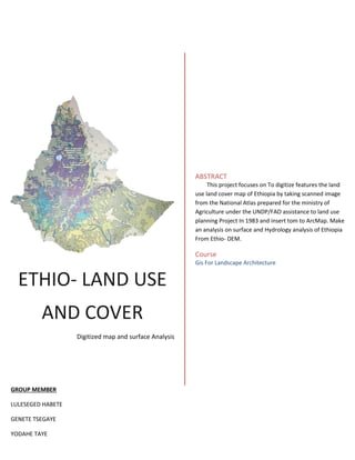
ETHIO- LAND USE
AND COVER
Digitized map and surface Analysis
ABSTRACT
This project focuses on To digitize features the land
use land cover map of Ethiopia by taking scanned image
from the National Atlas prepared for the ministry of
Agriculture under the UNDP/FAO assistance to land use
planning Project In 1983 and insert tom to ArcMap. Make
an analysis on surface and Hydrology analysis of Ethiopia
From Ethio- DEM.
Course
Gis For Landscape Architecture
GROUP MEMBER
LULESEGED HABETE
GENETE TSEGAYE
YODAHE TAYE

1 | P a g e
1
TABLE OF CONTENTS
i. ABSTRACT ……………………………………………………………………………...2
ii. ACKNOWLEDGMENT ……………………………………………………………………….3
1. OBJECTIVE OF THE STUDY…………………………………………………………………4
2. LOCATION MAP OF STUDY AREA ………………………………………………………...5
3. INTRODUCTION ……………………………………………………………………………..6
4. TYPE OF LAND USE LAND COVER ………………………………………………………..7
4.1. INTENSIVELY CULTIVATED LAND,
4.2. MODERATELY CULTIVATED LAND
4.3. AFRO-ALPINE AND SUB-AFRO-ALPINE VEGETATION
4.4. HIGH FOREST
4.5. WOODLAND,
4.6. RIPARIAN WOODLAND AND BUSHLAND
4.7. BUSHLAND AND SHRUB LAND
4.8. GRASSLAND
4.9. EXPOSED ROCK OR SAND SURFACE
4.10. SALT FLATS
4.11. SWAMPS AND MARSHES
4.12. WATER BODIES
4.13. URBAN AND BUILT-UP AREA
5. GEO-DATABASE PROCESS ………………………………………………………………11
6. DESCRIPTION OF DIGITALIZATION PROCESS ……………………………………… 11
7. SCANED ETHIOPIA LAND USE AND LAND COVER…………………………………..13
8. DIGITALIZED ETHIO LAND USE AND LAND COVER ………………………………..14
9. LAND USE AND LAND COVER MAP…………………………………………………….16
9.1.AFRO-ALPINE, WOOD & HIGH FOREST LAND MAP
9.2.RIPARIAN , BUSHLAND SHRUB LAND MAP
9.3.CULTIVATED LAND MAP
9.4.EXPOSED ROCK OR SALT FLAT LAND MAP
9.5.OPEN WATER, SWAMP – MARSHES & URBAN BUILT-UP LAND MAP
10. SPATIAL ANALYSIS ………………………………………………………………………21
11. ANALYSIS FROM SURFACE ……………………………………………………………..22
11.1. ASPECT
11.2. CONTOUR
11.3. SLOPE .
11.4. VIEW SHED
12. ANALYSIS FROM HYDROLOGY…………………………………………………………27
12.1. FILL
12.2. FLOW DIRECTION
12.3. FLOW ACCUMULATION
12.4. STREAM TO FEATURE
12.5. STREAM ORDER
12.6. BASIN
12.7. SNAP POUR POINT
12.8. WATER SHED
13. SUMMARY………………………………………………………………………………….36
14. REFERENCES. ……………………………………………………………………………...37

2 | P a g e
2
ABSTRACT
Land is the platform on which most human activities are performed and is the source of
many of materials needed for such activities. Land use/land cover is a significant element for the
interconnection of the human activities and environment. This report is used to identify the
different types of the land use and land cover and digitizing the Map in GIS. Digitalizing is the
process that helps in determining the land use and land cover properties with reference to land
use land cover map scanned from the National Atlas prepared for the ministry of Agriculture
under the UNDP/FAO assistance to land use planning Project In 1983. It helps in identifying the
land use land cover properties. The digitalizing map shows better accuracy of the properties. This
project also show the surface and Hydrology analysis from Ethio - DEM. This will help as to
understand

3 | P a g e
3
ACKNOWLEDGEMENT
First of all, we would like to express our thanks to our Almighty God Who helps us
and give strength to reach at this stage. We express our deepest gratitude to our instructors Dr.
Aramde Fetene and Mr Kibrom Hailu Since they assisted us in every steps of the project and
shared their knowledge that relates to the topic. Next we acknowledge our class mates and
friends since they allowed us to share their knowledge’s with us. We appreciate the help and
support of professionals that we have asked about factors for the project of Digitalizing the land
use land cover. Finally we appreciate our full cooperative participation in accomplishment of this
project in time.

4 | P a g e
4
GENERAL OBJECTIVE
This Project generally aimed at Digitalizing land use land cover map scanned from the
National Atlas prepared for the ministry of Agriculture under the UNDP/FAO assistance to land
use planning Project In 1983. Analyzed based on the Ethio-DEM file produce surface analysis
and hydrology analysis.
Finally will answer the following questions
 How to digitized manually From a Scanned image in GIS ?
 How to Analysis Spatially analysis in GIS Using Ethio -DEM?
 How to prepare Good GIS Map ?
 What do we understand from the land cover land use map ?
 What do we understand from spatial analysis ?

5 | P a g e
5
LOCATION MAP OF STUDY AREA

6 | P a g e
6
INTRODUCTION
Land use can be defined as the activity or activities for which land is used, and the same
land can support multiple uses. Land use identifies the purpose for what the land is committed;
which includes production of goods (such as crops, timber, animal products) and services (such
as recreation, public services and natural resources protection). It differs from land cover, which
describes the physical state of the land (vegetation type, soils, exposed rocks, water bodies. In
many classifications. Land use statistics provide information on the function and purpose for
which land is currently used and, if tracked over time, how land use changes. Appropriate land
use information requires consideration of three interrelated aspects or dimensions: information,
space, and time.
This project focused on Manual Digitizing In this method, the digitizer uses a digitizing
tablet (also known as a digitizer, graphics tablet, or touch tablet) to trace the points, lines and
polygons of a hard-copy map. This is done using a special magnetic pen, or stylus, that feeds
information into a computer to create an identical, digital map. Some tablets use a mouse-like
tool, called a puck, instead of a stylus. The puck has a small window with cross-hairs which
allows for greater precision and pinpointing map features. Also we will see Spatial Analyst
ArcGIS Spatial Analyst provides a broad range of powerful spatial modeling and analysis
features. You can create, query, map, and analyze cell-based raster data; perform integrated
raster/vector analysis; derive new information from existing data; query information across
multiple data layers; and fully integrate cell-based raster data with traditional vector data
sources.

7 | P a g e
7
4. TYPE OF LAND USE LAND COVER
4.1. LAND USE AND LAND COVER
This map is a generalized version of the 1:1,000,000 scale map of land use and land cover of
Ethiopia prepared for the ministry of Agriculture under the UNDP/FAO assistance to land use
planning Project In 1983. The following Description Of the mal or land use and land Cover types
shown on the map is also a summary from the text prepared to accompany the original map.
It contains 13 number of classes: these are, intensively cultivated land, Moderately cultivated
land , Afro-alpine and sub-afro-alpine vegetation ,High forest,
Wood land, Riparian woodland and bushland , Bushland and shrub land ,Grassland ,Exposed
rock or sand surface ,Salt flats ,Swamps and marshes, Water bodies, Urban and built-up area as
Shown on the table below
LAND USE/LAND COVER CATEGORIES
1 intensively cultivated land,
2 Moderately cultivated land
3 Afro-alpine and sub-afro-alpine vegetation
4 High forest
5 Woodland,
6 Riparian woodland and bushland
7 Bushland and shrub land
8 Grassland
9 Exposed rock or sand surface
10 Salt flats
11 Swamps and marshes
12 Water bodies
13 Urban and built-up area
Table 4 Land Use Land Cover categories adopted for study as per the explanation on the
National Map
4.2. INTENSIVELY CULTIVATED LAND
This type of land cover includes areas of intensively cultivated peasant mixed agriculture as well
as state farms. The intensively cultivated peasant mixed agriculture as well as accounts for about
10 3% of the total area of the country and

8 | P a g e
8
Includes land used for rain fed peasant cultivation of grains as well as sedentary peasant
livestock grazing. The major areas of this type of land use are found on the highlands of Tigray ,
Gonder, Gojam, Welo, Shewa, Aris and Parts of highland Harege, Northern Bale and Central
Welega . in these regions it is estimated that about 70% of the land is under annual crops, during
the rainy season and about 25% of mostly fallow land is used for grazing. The grazing land is
excessively overstocked and hardly any tree vegetation is visible .
The state farms account for nearly 0.2% of the total area of the country . they are found mostly in
the lowlands either as irrigated cultivation of mainly cotton , sugar cane and horticultural crops
or as rain fed cultivation of cereals.
The state farms account for nearly 0 Of the total area Of the country, They are found mostly in
the lowlands either as irrigated cultivation of mainly cotton, sugar cane and horticultural crops
Or as rain fed cultivation Of cereals.
4.3. MODERATELY CULTIVATED LAND
This accounts for about 12.5% Of the country and Includes land under rain fed peasant
cultivation of grains. Livestock grazing and browsing on unimproved Or fallow land and rain
fed peasant perennial crop cultivation of coffee, enset and chat, In contrast to the intensively
cultivated land patches of forest or bushes and large areas under natural vegetation are present.
This type of land use and land
Cover is found around the intensively cultivated land on most Of the highlands of Ethiopia. and
an estimated 50% of the total land is used for annual crops during the cropping season and about
is under fallow Or natural vegetation cover and is used for livestock grazing or browsing.
Perennial crop cultivation is more important in northern Sidamo, Kefa, Gamo Gofa, ilubabor,
southern Welega, southern Shew and in parts of highland Harerge than in the other parts of the
country in these regions ‘t is estimated that only about 25% of the land is under annual crops
during the cropping season.
4.4. AFRO-ALPINE AND SUB-AFRO-ALPINE VEGETATION
These account for some 0.2% of the total area of the country and are found above 3,200m
altitude They consist mostly of short shrub and heath vegetation used partly for sedentary
grazing and browsing: and, where the terrain permits, for some cultivation Of barley. The major
regions are the Simen highlands of Gonder, parts of southeastern Welo, parts of central Arsi and
northern Bale.
4.5. HIGH FOREST

9 | P a g e
9
The high forest region accounts for some 4.4% of the country and is found mostly in the
southwest and south. It consists of coniferous high forest in parts of central, southern and
southeastern highlands and of mixed high forest In the southwest.
The coniferous high forests consisting mostly Of podocarps graci” or and Junipers proceri have
been substance depleted from most of northern and central Ethiopia and only patches remain.
The mixed high forest of mostly broad-leafed species is found in most humid parts of the country
in the southwest ‘n parts of llubabor, Kefa, northern Gamo Gofa and in parts of Wetega where
the mean annual
rainfall is above 1.500m In the more dense high forest region. About Of the total land area is
under forest. About half of the total area designated as high forest. However, consists of
disturbed high forest where parts of the forest are cleared for settlement and cultivation of
perennial and annual crops. In these disturbed areas only about 60% of the land is forested.
4.6. WOODLAND
The woodlands are characterized by more discontinuous canopy and smaller trees than the high
forest region and account for some 2.5% of the total area of the country. Both the physiognomy
and the flora of the woodlands region vary from place to place and in many parts the woodland is
Interspersed With moderately cultivated land. More dense woodland is found on the drier
periphery of the high forest in the south and southwest. Here as much as 40% of the land may
consist Of patches Of forest and the main activity is livestock grazing and browsing as well as
rain fed peasant mixed agriculture. More open woodland consisting of mostly deciduous or
succulent trees with tall-grass under-story is found on the western edges Of Ethiopian highlands
in the west as well as in parts of the south and southeast. Much as 50% of this region may be
classified as grassland and pastoral activity is more dominant than in the dense wood land region.
Small portions of the country consisting of Planted eucalyptus trees around settlements is
included in the woodland region_ The largest area of eucalyptus wood-land is around Addis
Abeba.
4.7. RIPARIAN WOODLAND AND BUSHLAND
These occur along river banks and on floodplains and are important ‘n the semi-and and arid
parts Of the country where they are used for grazing and browsing and scattered seasonal crop
cultivation on some of the flood plains. They are found along most of the major rivers and
account for some 0.6% Of the area Of the country.
4.8. BUSHLAND AND SHRUB LAND

10 | P a g e
10
These account for about 21.4% of the area of the country and occupy the intermediate zone
between the humid and the semi-arid parts of the country. They are often intermixed With the
woodland and the moderately Cultivated land regions. Pastoral livestock grazing and browsing
and in some parts. Charcoal and incense harvesting are the main activities. The more dense
bushland occurs on the humid side of the region and consists of multi-stoned bushes. In the west.
Lowland bamboo bushland of pure stands of Oxyten-anthera Abyssinia is common, The shrub
land occurs on the semi-arid side and often consists of patches of shrubs interspersing grasslands
with some scattered low trees.
4.9. GRASSLAND
The grasslands region accounts for some 30.5% Of the area Of the country and is most extensive
in the western, southern and southeastern semi-arid lowlands of Ethiopia. On the more humid
side. Open grassland and grassland interspersed with some trees are common. In these regions
grass may account for as much as 90% of the area. In the drier parts. Patches of shrubs of bushes
are common and the proportion of grass is reduced to about 70% of the total area In these regions
pastoral livestock grazing and browsing and some incense and honey harvesting are common.
4.10. EXPOSED ROCK OR SAND SURFACE
These account for about 15.8% of the country and occur mostly in northern Hararghe, the
Danakil lowlands and along the Red Sea coast. Patches are also found in parts of Bale and
Hararghe lowlands in the southeast, the lower Omo valley and in parts of northwestern Eritrea.
In the northeast, the region consists mostly of recent lava flows with scattered small patches of
shrubs and scrub. In other parts it consists mostly of alluvial fans and depressions and partly of
overgrazed areas where the sparse vegetation of scattered scrub and grass allows some browsing
and grazing during the rain season.
4.11. SALT FLATS
The salt flats account for about 0.5% of the country and are most common in the Danakil
lowlands and along the Red Sea coast where the main activity is salt mining.
4.12. SWAMPS AND MARSHES

11 | P a g e
11
The swamps and marshes are Common around Some Of the lakes and in stream valleys and
depressions and account for about 0 of the country. The most extensive area occurs in the Baro ,
Akobo lowlands. The perennial swamps and marshes with grasses. sedges and scattered trees are
important grazing areas and bird wildlife sanctuaries. The seasonal swamps and marshes provide
grazing during the dry season and ‘n some places, as around lake Tana. They are used for
cultivating annual crops after the flood waters recede.
4.13. WATER BODIES
The water bodies include the large lakes Which account for about 0.5% of the area of the
country. This does not include the territorial waters of Ethiopia along the Red Sea coast and the
surfaces of the rivers. The large inland lakes are Abaya, Abilata, Awasa. Chamo, Koka,
Langeno, Shala, Tana and Ziway.
4.14. URBAN AND BUILT-UP AREA
Urban and built-up area is shown for Addis Abeba only since the areas occupied by other urban
centers are insignificant. The total built-up land is estimated at about 600 square kilometers
which is less than of the area of the Country.
5. GEO-DATABASE PROCESS
The Create Enterprise Geodatabase tool creates a database, storage locations, and a database user
to act as the geodatabase administrator and owner of the geodatabase. Functionality varies
depending on the database management system used. The tool grants the geodatabase
administrator privileges required to create a geodatabase, and then creates a geodatabase in the
database.
Visualize data
Once you have connected to your database from ArcGIS, you can view spatial data in a map by
dragging the table from your database connection to the map. If necessary, define a unique
identifier, spatial reference, and geometry type for spatial tables you add to the map.
When you drag a database feature class onto a map in an ArcGIS client, a query layer is created
automatically and is defined to include all columns of supported data types in the table. The first
row of the table is used to determine the geometry type (point, multipoint, line, or polygon),
spatial reference, and dimensionality (that is, 2D or 3D). If you don't want to use those
properties—for example, if you want to display the three-dimensional records in the table, but
the first record is two dimensional—you can alter the query layer definition.

12 | P a g e
12
Supported data types
To use the data with ArcGIS, the data types in your database table must map to those supported
by ArcGIS. If your table contains data types that ArcGIS does not support, ArcGIS will not
display the unsupported columns. When you move tables between databases or between
databases and geodatabases using ArcGIS, unsupported data types are not included in the
destination database. See DBMS data types supported in ArcGIS for a list of supported data
types per database management system.
Analyze data
Many geoprocessing tools can be used to analyze data in a database. Just be aware that if the tool
adds records to an existing table, the table must contain a unique identifier that is maintained by
the database.
When doing spatial analysis on large feature classes, though, it may be more efficient to write
queries that use the database's native SQL functions in the query layer interface. These queries
are processed in the database.
6. DESCRIPTION OF DIGITALIZATION PROCESS
How to digitize features on a surface in ArcGlobe
Steps:
 Start ArcGlobe and add the 2D feature class (point, line, polygon) you want to create new
features for.
By default, the layer is automatically added to the draped category in the table of contents.
Add the surface data that you want to drape the features on, for example, a TIN or raster or an
elevation service.
 Optionally add any imagery that you want to use as the backdrop for digitizing from. You
only require a surface layer to digitize from, but sometimes an image draped on the
surface can make the view more realistic. The image's layer properties will need to be
draped on the surface of the globe.
 The surface will act as the elevation source for any newly created features.
 On the 3D Editor toolbar, click the 3D Editor drop-down list and click Start Editing.
If the layers in your table of contents come from more than one source, you may be
prompted to choose the layer or workspace to edit.
 If you prefer, now would be a good time to open the Snapping Environment window to
set snapping properties. Open the window by clicking 3D Editor, expand the Snapping
side menu and click Snapping window.

13 | P a g e
13
 Choose a feature template and select the edit construction tool from the Create Features
window to begin creating new features.
 Click the surface to place vertices for new features. For polylines and polygons, double-
click the last vertex to finish the sketch.When you are finished digitizing features, click
3D Editor and click Stop Editing. You will be prompted to save or reject your edits.
7. SCANED ETHIOPIA LAND USE AND LAND COVER

14 | P a g e
14
8. DIGITALIZED ETHIO LAND USE AND LAND COVER

15 | P a g e
15
IMAGE PRE-PROCESSING AND PROCESSING
Image enhancement To increase the quality of image classification so enhancement technique is
must. The most commonly used image enhancement techniques are histogram equalization,
radiometric correction, contrast stretching… on this histogram equalization is used for the
images.
The land Use land cover map gained from the atlas map scanned and georeferenced
using points and a map gained from the Ethiopian region. We use 9 points to georeferenced and
make the map at its exact reference point in the globe. After all these things have done the
creation of new feature data set as a polygon and new class features as a polygon. All the new
feature classes are polygon features. Because we are working on the land/use land cover aspect
and it is described interims of polygon. The features are Cultivated Land, Intensively cultivated
land, Moderately cultivated Land, Afro -Alpine vegetation, Wood land, High Forest, Riparian
Vegetation, Bush land, Bush Shrub Land, Exposed Rock, Salt Flat lands, open water, swamp and
marshes and the urban built up area lands as well as the Boundary of Ethiopia as well. All the
above features are digitized from the georeferenced map one by one. Not only digitizing the
features but also calculate the relative area and perimeter of each feature in kilometer square and
kilometer respectively. After having all these maps were produced showing all the land use and
land-cover of the data. The maps were produced in category that goes together. That is Map of
Land use /Land cover, Map of afro alpine, wood and high forest lands, map of Bush and Shrub
land, Map of Cultivated Land, Intensive and Moderately cultivated land and lastly Map of
exposed rock and flat salt lands.

16 | P a g e
16
9. LAND USE AND LAND COVER MAP
9.1. AFRO-ALPINE, WOOD & HIGH FOREST LAND MAP
Most of the wood land cover
exist western part of Ethiopia

17 | P a g e
17
9.2. RIPARIAN , BUSHLAND SHRUB LAND MAP
Most of Riparian , bush-shrub
and Bush Land existed in southeast direction

18 | P a g e
18
9.3. CULTIVATED LAND MAP

19 | P a g e
19
9.4. EXPOSED ROCK LAND MAP

20 | P a g e
20
9.5. OPEN WATER, SWAMP – MARSHES & URBAN BUILT-UP LAND MAP

21 | P a g e
21
10. SPATIAL ANALYST
ArcGIS Spatial Analyst provides a broad range of powerful spatial modeling and analysis
features. You can create, query, map, and analyze cell-based raster data; perform integrated
raster/vector analysis; derive new information from existing data; query information across
multiple data layers; and fully integrate cell-based raster data with traditional vector data
sources.
With ArcGIS Spatial Analyst, you can:
 Derive new information from existing data
Apply Spatial Analyst tools to create useful information—for example, derive distance from
points, polylines, or polygons; calculate population density from measured quantities at certain
points; reclassify existing data into suitability classes; or create slope, aspect, or hillshade outputs
from elevation data.

22 | P a g e
22
11. ANALYSIS FROM SURFACE
STEPS
1. ANALYSIS FROM SURFACE
We have extracted the following, from the surface in spatial analyst tool.
Aspect
Input - Ethio-DEM
Contour
Input - Ethio-DEM
Slope
Input – Ethio-DEM
View shed
Input – Ethio-DEM
11.1. ASPECT

23 | P a g e
23
Derives aspect from a raster surface. The aspect identifies the downslope direction of the
maximum rate of change in value from each cell to its neighbors.
Aspect can be thought of as the slope direction. The values of the output raster will be the
compass direction of the aspect.
Usage
 Aspect is the direction of the maximum rate of change in the z-value from each cell in a
raster surface.
 Aspect is expressed in positive degrees from 0 to 359.9, measured clockwise from north.
 Cells in the input raster that are flat—with zero slope—are assigned an aspect of -1.
 If the center cell in the immediate neighborhood (3 x 3 window) is NoData, the output is
NoData.
 If any neighborhood cells are NoData, they are first assigned the value of the center cell,
then the aspect is computed.
Aspect identifies the downslope direction of the maximum rate of change in value from each cell
to its neighbors. It can be thought of as the slope direction. The values of each cell in the output
raster indicate the compass direction that the surface faces at that location. It is measured
clockwise in degrees from 0 (due north) to 360 (again due north), coming full circle. Flat areas
having no downslope direction are given a value of -1.
The value of each cell in an aspect dataset indicates the direction the cell's slope faces.
Conceptually, the Aspect tool fits a plane to the z-values of a 3 x 3 cell neighborhood around the
processing or center cell. The direction the plane faces is the aspect for the processing cell.
The following diagram shows an input elevation dataset and the output aspect raster.

26 | P a g e
26
11.4. VIEW SHED

27 | P a g e
27
12. ANALYSIS FROM HYDROLOGY
The Hydrology tools are used to model the flow of water across a surface. Information about the
shape of the earth's surface is useful for many fields, such as regional planning, agriculture, and
forestry. These fields require an understanding of how water flows across an area and how
changes in that area may affect that flow.
When modeling the flow of water, you may want to know where the water came from and where
it is going. The following topics explain how to use the hydrologic analysis functions to help
model the movement of water across a surface, the concepts and key terms regarding drainage
systems and surface processes, how the tools can be used to extract hydrologic information from
a digital elevation model (DEM), and sample hydrologic analysis applications.
STEP
We have extracted the following Stream features
Fill
Input – Ethio-DEM
Flow direction
Input - Fill
Flow accumulation
Input – Flow direction
Arc toolbox – Spatial analyst tool -- Map Algebra -- Raster Calculator --- >500 -- (A)
Arc toolbox – conversion tool --- from Raster ---- Raster to Polyline --- (B)
Stream to feature
Input – Raster Calculated (A)
– Flow direction
Stream link
Input – Raster to Polyline (B)
– Flow direction
Stream order
Input – Stream feature
– Flow Direction
Basin
Personal Geo-Database --- Feature class --- Point --- (C)
Locating the junctions of big streams from our stream order map
Snap Pour point
Input – Point (C)
– Flow accumulation
Water shed

28 | P a g e
28
– Pour point
12.1. FILL

29 | P a g e
29
12.2. FLOW DIRECTION
Usage
The output of the Flow Direction tool is an integer raster whose values range from 1 to 255. The
values for each direction from the center are the following:
Flow Direction codes
For example, if the direction of steepest drop was to the left of the current processing cell, its
flow direction would be coded as 16.

30 | P a g e
30
If a cell is lower than its eight neighbors, that cell is given the value of its lowest neighbor, and
flow is defined toward this cell. If multiple neighbors have the lowest value, the cell is still given
this value, but flow is defined with one of the two methods explained below. This is used to filter
out one-cell sinks, which are considered noise.
If a cell has the same change in z-value in multiple directions and that cell is part of a sink, the
flow direction is referred to as undefined. In such cases, the value for that cell in the output flow
direction raster will be the sum of those directions. For example, if the change in z-value is the
same both to the right (flow direction = 1) and down (flow direction = 4), the flow direction for
that cell is 1 + 4 = 5. Cells with undefined flow direction can be flagged as sinks using the Sink
tool.
If a cell has the same change in z-value in multiple directions and is not part of a sink, the flow
direction is assigned with a lookup table defining the most likely direction. See Greenlee (1987).
The output drop raster is calculated as the difference in z-value divided by the path length
between the cell centers, expressed in percentages. For adjacent cells, this is analogous to the
percent slope between cells. Across a flat area, the distance becomes the distance to the nearest
cell of lower elevation. The result is a map of percent rise in the path of steepest descent from
each cell.
When calculating the drop raster in flat areas, the distance to diagonally adjacent cells (1.41421 *
cell size) is approximated by 1.5 * cell size for improved performance.
With the Force all edge cells to flow outward parameter in the default unchecked setting
(NORMAL in Python), a cell at the edge of the surface raster will flow toward the inner cell with
the steepest drop in z-value. If the drop is less than or equal to zero, the cell will flow out of the
surface raster.

31 | P a g e
31
The Flow Accumulation tool calculates accumulated flow as the accumulated weight of all cells
flowing into each downslope cell in the output raster. If no weight raster is provided, a weight of
1 is applied to each cell, and the value of cells in the output raster is the number of cells that flow
into each cell.
In the graphic below, the top left
image shows the direction of travel
from each cell and the top right the
number of cells that flow into each
cell.

32 | P a g e
32
12.4. STREAM TO FEATURE
The algorithm used by the Stream to Feature tool is designed primarily for vectorization of
stream networks or any other raster representing a raster linear network for which directionality
is known.
The tool is optimized to use a direction raster to
aid in vectorizing intersecting and adjacent cells. It
is possible for two adjacent linear features of the
same value to be vectorized as two parallel lines.
This is in contrast to the Raster To Polyline tool,
which is generally more aggressive with
collapsing the lines together.
To visualize this difference, an input stream
network is shown below, with the simulated
Stream to Feature output compared to the Raster
To Polyline output.

33 | P a g e
33
12.5. STREAM ORDER
For example, first-order streams are dominated by overland flow of water; they have no
upstream concentrated flow. Because of this, they are most susceptible to non-point source
pollution problems and can derive more benefit from wide riparian buffers than other areas of the
watershed.
12.6. BASIN
The drainage basins are delineated within the analysis window by identifying ridge lines between
basins. The input flow direction raster is analyzed to find all sets of connected cells that belong
to the same drainage basin. The drainage basins are created by locating the pour points at the

34 | P a g e
34
edges of the analysis window (where water would pour out of the raster), as well as sinks, then
identifying the contributing area above each pour point. This results in a raster of drainage
basins. The best results will be obtained if when the input Flow Direction raster was created, the
Force all edge cells to flow outward option (FORCE in Python) was enabled. All cells in the
raster will belong to a basin, even if that basin is only one cell.
12.7. SNAP POUR POINT
The Snap Pour Point tool is used to ensure the selection of points of high accumulated flow when
delineating drainage basins using the Watershed tool. Snap Pour Point will search within a snap
distance around the specified pour points for the cell of highest accumulated flow and move the
pour point to that location.
If the input pour point data is a point feature class, it will be converted to a raster internally for
processing.
The output is an integer raster when the original pour point locations have been snapped to
locations of higher accumulated flow.
When there is only one input pour point location, the extent of the output is that of the
accumulation raster. If there is more than one pour point location, the extent of the output is
determined by the settings in the Output extent environment.
When specifying the input pour point locations as feature data, the default field will be the first
available valid field. If no valid fields exist, the ObjectID field (for example, OID or FID) will be
the default.

35 | P a g e
35
12.8. WATER SHED
A watershed is the upslope area that contributes flow—generally water—to a common outlet as
concentrated drainage. It can be part of a larger watershed and can contain smaller watersheds,
called sub basins. The boundaries between watersheds are termed drainage divides. The outlet, or
pour point, is the point on the surface at which water flows out of an area. It is the lowest point
along the boundary of a watershed.

36 | P a g e
36
Findings of the LU/LCC analysis under different institutional arrangements between 2006
and 2016 showed expansion of agriculture/settlement and reduction of woodland and forests
under all institutions, but with differing rates. The rate of agriculture/settlement expansion was
high in lowland Kebele under Wereda land administration with followed by Kebele under the
national park with (290 ha/year) and Kebele under PFM in mid lands. In contrast rate of
agriculture/settlement expansion was much smaller in the highland Kebele under the Wereda
institution.
On the contrary the rate of deforestation is low in forests and woodlands managed under
PFM and PRM institutional arrangements. LU/LCC in the BER is a result of different
interactions between proximate and underlying causes. The major proximate driving forces of
LU/LCC in the Ethiopia are expansion of agriculture, fire, illegal logging and fuel wood
extraction, overgrazing and illegal and unplanned settlement. On the other hand from a range of
demographic, economic, technological, policy and institution, socio-cultural and biophysical
factors underlying drivers of LU/LCC are identified by key informant and focus group
discussants of this study. However population growth, poverty and food insecurity, gradual
change in the economic activities of communities in the area from pure pastoralist to agro-
pastoralist, weak law enforcement and drought appear to explain a large part of underlying
causes.

37 | P a g e
37
14.REFERENCES
1. National Atlas prepared for the ministry of Agriculture under the UNDP/FAO assistance to
land use planning Project In 1983. PG 10-11
2. Ethio_Dem From Chair Of Urban Planning in Eiabc
3. Arch Gis 10.5 Help

Land use and land cover of Ethiopia

Recommended

Recommended

More Related Content

What's hot

What's hot (20)

Similar to Land use and land cover of Ethiopia

Similar to Land use and land cover of Ethiopia (20)

Recently uploaded

Recently uploaded (20)

Land use and land cover of Ethiopia