SlideShare a Scribd company logo
1 of 9
Download to read offline
Development and Practical Application of Petroleum and Dispersant
Interspecies Correlation Models for Aquatic Species
Adriana C. Bejarano*,†
and Mace G. Barron‡
†
Research Planning, Inc., 1121 Park Street, Columbia, South Carolina 29201, United States
‡
U.S. Environmental Protection Agency, Gulf Ecology Division, 1 Sabine Island Drive, Gulf Breeze, Florida 32561, United States
*S Supporting Information
ABSTRACT: Assessing the acute toxicity of oil has generally relied on
existing toxicological data for a relatively few standard test species, which has
limited the ability to estimate the impacts of spilled oil on aquatic
communities. Interspecies correlation estimation (ICE) models were
developed for petroleum and dispersant products to facilitate the prediction
of toxicity values to a broader range of species and to better understand
taxonomic differences in species sensitivity. ICE models are log linear
regressions that can be used to estimate toxicity to a diversity of taxa based on
the known toxicity value for a surrogate tested species. ICE models have only
previously been developed for nonpetroleum chemicals. Petroleum and
dispersant ICE models were statistically significant for 93 and 16 unique
surrogate-predicted species pairs, respectively. These models had adjusted
coefficient of determinations (adj-R2
), square errors (MSE) and positive slope
ranging from 0.29 to 0.99, 0.0002 to 0.311, and 0.187 to 2.665, respectively. Based on model cross-validation, predicted toxicity
values for most ICE models (>90%) were within 5-fold of the measured values, with no influence of taxonomic relatedness on
prediction accuracy. A comparison between hazard concentrations (HC) derived from empirical and ICE-based species
sensitivity distributions (SSDs) showed that HC values were within the same order of magnitude of each other. These results
show that ICE-based SSDs provide a statistically valid approach to estimating toxicity to a range of petroleum and dispersant
products with applicability to oil spill assessment.
■ INTRODUCTION
Assessments of the potential toxicological effects of physically
or chemically dispersed oils and dispersants have commonly
relied on relatively few toxicity tests for a limited number of
aquatic species, primarily standard test species. In most cases,
the sensitivity of species of concern is unknown, making
informed decisions challenging. One approach to addressing
uncertainty in species sensitivity has been the development and
application of interspecies correlation estimation models
(ICE),1
which are log−linear regressions between the acute
toxicity of two species for many paired toxicity data. These
models can generate acute toxicity estimates by extrapolating
known toxicity values from a surrogate species to species with
unknown toxicity values. While these models are available for
many chemicals,2−5
these have not been developed for
petroleum or dispersant products. ICE models can be used to
generate species sensitivity distributions (SSDs),2,6,7
which are
cumulative distributions of toxicity data (e.g., median lethal,
LC50, and effects concentrations, EC50) that allow for
comparisons of the relative sensitivities of across species.8
SSDs have been used to establish protective levels to specific
chemicals9
by deriving hazard concentrations (HC) assumed to
protect a wide number of species with varying sensitivities. ICE-
based SSDs have been developed for a number of chemicals,2,6,7
and have been shown to produce HC values similar to those
used to derive water quality criteria.6
Recent research has shown that existing data from stand-
ardized toxicity tests can be used to develop oil-specific
SSDs,10−13
but species diversity is extremely limited compared
to single compounds.2,4,5
The objectives of the current study
were to determine if petroleum and dispersant-specific ICE
models could be developed and used to generate SSDs and
HC5 values with acceptable uncertainty, and to determine
associations between taxonomic relatedness and species
sensitivity.4
Previous studies have documented variability in
test results attributable to differences in test conditions and
exposure media prepared from the same source oil and/or
dispersants.14−17
Therefore, this study focused on two distinct
categories of studies (spiked and continuous exposure) that
reported measured aqueous exposure concentrations of
petroleum products (primarily light and medium crude oils)
and several oil spill dispersants (primarily Corexits). The
models and approach presented here can be used to estimate
toxicity to a broad range of species and assemblages which
Received: October 25, 2013
Revised: March 17, 2014
Accepted: March 21, 2014
Published: March 28, 2014
Article
pubs.acs.org/est
© 2014 American Chemical Society 4564 dx.doi.org/10.1021/es500649v | Environ. Sci. Technol. 2014, 48, 4564−4572
should facilitate the development of protective environmental
concentrations and improved assessment of the potential
consequences of oil spills and dispersant use.
■ EXPERIMENTAL SECTION
Petroleum and Dispersant Toxicity Data Sources. The
primary data source used in the development of ICE models
came from a recently developed toxicity database,18
which
contains quantitative information on the acute toxicity of crude
oils and dispersants from publically available literature. This
database was developed following a quality assurance and
quality control (QA/QC) plan similar to that of a related
database.19
QA/QC procedures included an evaluation of each
original data source, removal of duplicate information, and an
evaluation of currently accepted scientific names.
Two types of data sets were queried and used in the
development of ICE models: petroleum hydrocarbon and
dispersant toxicity data. The petroleum hydrocarbon data set
was comprised of toxicity data (LC50 and EC50) for aquatic
species (primarily fish and crustaceans) derived from aqueous
exposures to physically dispersed (i.e., water accommodated
fractions; WAF) or chemically dispersed (i.e., enhanced water
accommodated fractions; CEWAF) oil. These toxicity data
were generated using a variety of oils under various weathering
stages, but most data were from light (e.g., Chirag, Forties,
South Louisiana, Venezuelan) and medium (e.g., Alaska North
Slope, Forcados, Kuwait, Prudhoe Bay) crude oils (42 oils of 48
total oils). Only studies that reported LC50 and EC50 toxicity
values on the basis of measured concentrations of analytes in
the aqueous exposure media were included in the development
of these models. While rigorous data selection for petroleum
hydrocarbons focused on test results reported on the basis of
measured total hydrocarbon content (THC; including C6−
C36 carbon chains; 72% of the entire data set), other reported
metrics (total polycyclic aromatic hydrocarbons, TPAHs; sum
of PAHs and alkyl homologue groups) were also included. This
data set did not include results from studies reporting effects
concentrations for specific THC carbon chains or PAH
analytes. Petroleum ICE models were developed using over
1500 paired data points for a total of 136 unique species pairs.
The dispersant data set was comprised of toxicity data (LC50
and EC50) for aquatic species exposed to dispersants, almost
exclusively Corexit 9500 and Corexit 9527 (36% and 33% of
the entire data set respectively). Toxicity data for other
dispersants (Corexit 7500; Corexit 7664; Corexit 9552;
Nokomis; SlickAWay) were also included. Only studies
reporting LC50 and EC50 toxicity values on the basis of
measured dispersant concentrations in the exposure media were
included in model development. Dispersant ICE models were
developed using 286 paired data points for a total of 38 unique
species pairs.
The majority of data included here were derived from
standard toxicity tests, including 96 h (65% of the entire data
set) and constant static (76% of the entire data set) laboratory
exposures. To develop petroleum and dispersant ICE models,
surrogate and predicted species were paired from the same
original data source. Pairing of surrogate and predicted species
toxicity data was done only when tests for both species were
performed under the same exposure conditions (i.e., same oil or
dispersant product, exposure regime, analytical methods in
chemical characterization), but with data independently
collected for each species. A complete list of data sources and
core data are provided in the Supporting Information (SI)
material.
Model Development and Verification. Because of the
number of steps involved in the development, selection,
verification and application of ICE models, a diagram is
provided (SI Figure S1) to facilitate the understanding of the
approach presented here. As several statistical methods were
used, the readers are encouraged to refer to key statistical
references20,21
including those describing the development of
ICE models.2,5
Linear regression models were developed for
each pair of species in both, the petroleum hydrocarbon and
dispersant database, containing at least 4 data points. These
linear models are described by Log Pi = β0 + β1 × Log (Si),
where Pi is the acute toxicity of the predicted species, β0 and β1
are the intercept and slope, respectively, and Si is the acute
toxicity of the surrogate species, where both the independent
and dependent variables are random and independent of each
other.22
The slope represents change in the response of toxicity
values of the predicted species per unit change in the toxicity
values of the surrogate species, where a slope of approaching 1
indicates a similar response between two species. Only ICE
models (p-value < 0.05) that passed both the F-test for the
overall fit of the regression equation and the t test for the slope
parameter significantly different from 0, were included in
further analyses. Prior to model validation, statistically
significant models were evaluated for potential influential data
via regression diagnostics analyses.20
The reliability and
predictive power of statistically significant ICE models with at
least 2 degrees of freedom was assessed using a leave-one-out
cross-validation technique.23,24
Briefly, each data set was split
into K subsets, equal to the number of pairs within each data
set, and models fitted K times, each time leaving out one data
subset from the larger training data. For each reduced data set,
toxicity values of the predicted species were calculated and
responses for the deleted subset predicted from the model.
Model uncertainty of the estimated toxicity value was calculated
via the cross-validation success rate (or 1-bias corrected
misclassification error or sum of the square difference between
observed and estimated values), which is an estimate of
generalized error. Taxonomic relatedness for each surrogate
and predicted species was assigned a numeric distance value4
(from same genus = 1 to same domain = 7), and model
prediction accuracy assessed as a function of taxonomic
distance.
Practical Application of ICE Models. Regression
parameters of statistically significant ICE models were used
to estimate toxicity values of several predicted species, using the
known toxicity of petroleum hydrocarbons or dispersants for
one or more surrogate species as the model input. In all
instances, input data for surrogate species were independent of
the data used to develop ICE models.10,18
Surrogate species
included Americamysis bahia (mysid shrimp), Holmesimysis
costata (kelp forest mysid), Menidia beryllina (inland silverside)
and Atherinops affinis (topsmelt). ICE-based SSDs were
generated for each category of petroleum or dispersant product
using the ICE estimated toxicity values, and in all cases the
minimum acceptable number of species on an SSD was set to
five. The petroleum product categories included light crude oils
(>31.1°API) (Forties, South Louisiana, Venezuelan crudes)
and medium crudes (22.3−31.1°API) (Alaska North Slope,
Arabian Medium, Kuwait and Prudhoe Bay crudes), while the
dispersant categories included Corexit 7664, Corexit 9500, and
Corexit 9527. Hazard concentrations (HC) assumed to be
Environmental Science & Technology Article
dx.doi.org/10.1021/es500649v | Environ. Sci. Technol. 2014, 48, 4564−45724565
protective of 99% or 95% of the species in the SSD (i.e., HC1
and HC5, respectively) were computed from the modeled SSD
function. All SSDs and HC values were derived using an
approach described elsewhere.25
Briefly, toxicity values were
fitted to a log-normal distribution function, and SSDs randomly
resampled 2000 times to derive the HC1 and HC5 values and
their associated 95% confidence intervals (95% CI). Only SSDs
that passed goodness of fit tests (α = 0.01) (the Anderson−
Darling for SSDs with >7 species, and the Kolmogorov−
Smirnov test statistics) were included in these analyses. SSDs
were also generated using empirical data for the same categories
of petroleum products and dispersants, as well as using a
combination of empirical data and ICE-based toxicity values.
SSDs with empirical data were generated by calculating the
geometric mean of all toxicity values available for each unique
species. The geometric was used because it gives less weight to
influential data or potentially outliers, leading to conservative
estimates.8
To determine if ICE-based SSDs are a viable
alternative to the estimation of SSDs where toxicity data are
limiting, ICE-based SSDs were compared to empirically based
SSDS using log-likelihood statistics.21
This approach compares
the log-likelihood values of individual SSDs (e.g., M. beryllina
ICE-based and empirical data) with the fitted SSDs of the
combined (pooled) model (e.g., M. beryllina ICE-based plus
empirical data), testing the hypothesis (via the chi-square
statistic) that these SSDs are derived from the same fitted log-
normal curve. The same approach was used to compare ICE-
based SSDs pairs. All the analyses above were performed using
the R statistical platform (v. 2.13.2).22
■ RESULTS
Model Development and Verification. A total of 93
petroleum ICE models for 29 surrogate species, and 16
dispersant ICE models for seven surrogate species were
statistically significant (p-value <0.05 for both, the F-test for
the overall fit and the t test for the slope parameter) (SI Tables
S1−S3, Figures S2 and S3). Models lacking significance
typically had limited paired data (22 petroleum and 5
dispersant ICE models with <5 paired data points) limiting
their use in further analyses.
The validity of statistically significant models was verified
using standard regression diagnostics procedures.20
Visual
examination of the standardized residuals of each significant
model (Figure 1, left panel) showed that all residuals fell within
a horizontal band centered on 0, indicating that the variance of
the error term was constant. No obvious outliers were detected
(±4 standardized residual values). Diagnostic analyses also
indicated that the error term did not depart substantially from a
normal distribution (Figure 1, right panel), as the coefficient of
determination (R2
) between residuals and quantiles for
petroleum and dispersant ICE models were greater (0.997
and 0.991, respectively) than those of the critical R2
value
(0.985) (α = 0.05; n ≥ 100).26
A moderate departure from
normality was noted at the end tails of the distributions,
particularly for petroleum ICE models (14 data points) but was
considered minimal because removal of these data points did
not cause major changes in fitted values. In all cases, the
absolute change between fitted values with and without
potentially influential points ranged from 4 to 11% indicating
no disproportional influence on fitted values.
Statistically significant models had an adjusted coefficient of
determination (adj-R2
) ranging from 0.29 and 0.99, a Mean
Square Error (MSE; a measure of fit) ranging from 0.0002 to
0.311, and a positive slope ranging from 0.187 to 2.665 (SI
Tables S2 and S3). Examination of model parameter viability
shows that 92% of all intercepts were between −0.75 and 0.75,
and that 85% of all slopes were between 0.5 and 1.5. This
relatively narrow variability suggests similarities across most
models. Notable exceptions, where both the slope and intercept
of the same model were outside these ranges included (1) the
petroleum ICE models for the surrogate-predicted pairs
Calanus sinicus- Paracalanus aculeatus (both copepods species),
Cyprinodon variegatus (sheepshead minnow)-A. bahia, and
Pontogammarus maeoticus (amphipod)-Calanipeda aquae dulcis
(copepod); and (2) the dispersant ICE models for the pairs C.
variegatus-A. bahia, A. affinis-H. costata, and A. affinis-
Macrocystis pyrifera (giant kelp). In these deviating cases,
except pairs involving A. affinis, the predicted species was
generally more sensitivity than the surrogate species, but in all
cases MSE were small (below 0.16).
Figure 1. Diagnostic analyses of homogeneity of variances (left) and normality (right) for petroleum and dispersant ICE models.
Environmental Science & Technology Article
dx.doi.org/10.1021/es500649v | Environ. Sci. Technol. 2014, 48, 4564−45724566
The reliability and predictive power of statistically significant
models was further assessed by identifying the MSE cutoff
associated with a-priori cross-validation success rates of 85%
and 95%,5
assumed to have moderate and high reliabilities,
respectively (Figure 2). MSE cutoffs for petroleum and
dispersant models were 0.126 and 0.04, respectively. Over
half of the petroleum ICE models (54 models) had MSEs
≤0.04, while over 30% (32 models) had MSEs between 0.04
and 0.126. By comparison, dispersant ICE models were equally
distributed among MSE cutoffs, suggesting that petroleum ICE
models may be more robust.
The high cross-validation success rate (a measure of
predictive power) was consistent with the agreement between
predicted and observed values for both ICE models types
(Figure 3). For petroleum ICE models, 98% of the predicted
values were within 5-fold difference of the observed data, with
most values (92%) being within 2-fold difference of the
observed data. There was no influence of taxonomic relatedness
on prediction accuracy (p-value >0.05), and mean fold-
difference values across taxonomic distances ranged from 1.00
to 1.38 (SI Figure S4). Only 0.5% of predicted values (seven
observations) were >10-fold difference from the observed
values. These outliers occurred only in the M. beryllina- A. bahia
(taxonomic distance = 6), Daphnia magna (water flea)- Artemia
salina (brine shrimp) (taxonomic distance=4), and A. bahia- M.
beryllina surrogate- predicted pairs (3, 3, and 1 observations,
respectively). For dispersant ICE models, 99% of the predicted
values were within 5-fold difference of the observed data, with
most values (88%) being within 2-fold of the observed data.
There was no influence of taxonomic relatedness on prediction
accuracy (p-value >0.05), and mean fold-difference values were
1.29 and 1.14 for taxonomic distances 6 and 7, respectively.
The largest fold difference of 7 occurred in the A. bahia- M.
beryllina surrogate- predicted pair.
Practical Application of ICE Models. Toxicity data for
several petroleum products from an analysis independent of the
research presented here10
were used to verify the applicability
of ICE models. Two sets of SSD were developed using ICE
models for A. bahia and M. beryllina as the surrogate species,
with input surrogate concentrations from Barron et al.10
The
first set of SSDs used all ICE models regardless of their
reliability, while the second set used only ICE models with
MSE <0.12. Statistical comparison of SSDs via (using the log-
likelihood),21
showed that these two types of SSDs for several
petroleum products and for both surrogate species, were not
significantly different from each other (p-value >0.05). This
indicates that exclusion of the least reliable models did not
influence the shape of the SSD. No statistically significant
differences were also found between A. bahia and M. beryllina
ICE-based SSDs (p-value >0.05), or between either of these
two ICE-based SSDs and empirical SSDs10
(p-value >0.05;
Figure 4). Estimated petroleum hydrocarbon HC5s from ICE-
based SSDs were in general agreement with those derived from
SSDs using empirical data10
(SI Table S5), though values from
M. beryllina as the surrogate were generally larger (up to a 6
fold larger) than those calculated from empirical data.
A second verification approach utilized empirical toxicity data
for physically and chemically dispersed combined from
constant and spiked exposures, as well as toxicity data for
Corexit 9500 and Corexit 9727,18
which were used to generate
SSDs (Figure 5). The selection of these data was driven by the
fact that these SSDs shared data for two surrogate species: H.
costata and A. bahia. SSDs were derived using all ICE models
Figure 2. Assessment of model reliability based on the relationship
between model mean square error (MSE) and cross-validation success
rate for both, petroleum and dispersant ICE models.
Figure 3. Comparison of observed and ICE-predicted toxicity values for petroleum hydrocarbons and dispersants. The solid line represents the 1:1
line (equal toxicity), while the dotted lines represent a 5-fold difference between these values. Bar chart on the right, display the fold-difference
between observed and ICE-predicted toxicity values.
Environmental Science & Technology Article
dx.doi.org/10.1021/es500649v | Environ. Sci. Technol. 2014, 48, 4564−45724567
for these surrogate species regardless of model reliability.
Because there were insufficient paired surrogate-predicted ICE
models for the same surrogate species to generate SSDs for
dispersants (five species minimum), predicted ICE model
concentrations were combined for H. costata and A. bahia.
Curve comparison of empirically and ICE-based SSDs, using
log-likelihood, showed no statistically significant differences
between A. bahia and H. costata ICE-based SSDs (p-value
>0.05), or between either of these two ICE-based SSDs and
empirical SSDs10,18
(p-value >0.05), with one exception: the H.
costata ICE-based SSDs and the empirical SSDs18
for constant
exposures to dispersed oil (p-value = 0.01; Figure 5). In most
cases, ICE-based models with H. costata and A. bahia as
surrogates, produced smaller HC5s indicative of a slight model
bias toward overprotection of aquatic species. In all cases, HC5s
from ICE-based SSDs were within the same order of magnitude
as HC5s from empirical SSDs. HC5s for Corexit 9500 and
Corexit 9727 from ICE-based SSDs were also similar to those
reported by Barron et al.10
Hazard concentrations (96 h HC1 and HC5) were estimated
for fresh petroleum and dispersant products for which data, on
the basis of measured concentrations, were available from
constant static and spiked flow-through exposures (Table 1).
These hazard concentrations were estimated using ICE-based
SSD with models from each of two surrogate species (A. bahia
and M. beryllina). An additional set of SSDs was also
constructed by combining all available empirical data plus
Figure 4. Comparison between species sensitivity distribution (SSD)
curves for all petroleum products from Barron et al.10
(dashed line),
and SSDs derived using all ICE models, regardless of their reliability,
with A. bahia (black dots and lines) and M. beryllina (blue dots and
lines) as the surrogate species. These curves are not significantly
different (p-value >0.05) from each other.
Figure 5. Comparison between physically and chemically dispersed oil (top), and dispersant (bottom) species sensitivity distribution (SSD) using
empirical18
and ICE-based models (red dots and lines; red dashed line from Barron et al.10
for dispersants only). SSDs using empirical data for
dispersed oil were developed for constant and spiked exposures separately. SSDs were derived using all ICE models regardless of their reliability with
A. bahia (black dots and lines) and H. costata (blue dots and lines) as surrogate species, combining models for these two species for dispersant SSDs
(black lines). Within panels, SSDs are not significantly different (p-value > 0.05) from each other, except for the comparison of H. costata ICE-based
SSDs and the empirical SSDs for constant exposures to dispersed oil (p-value = 0.01; top left).
Environmental Science & Technology Article
dx.doi.org/10.1021/es500649v | Environ. Sci. Technol. 2014, 48, 4564−45724568
ICE toxicity values for one or more surrogate species (A. bahia,
H. costata, M. beryllina and A. affinis), keeping the smallest
predicted value for each unique predicted- species (SI Figure
S5). Starting concentrations for surrogate species were those of
studies reporting measured toxicity data,14,15,27−37
and excluded
from model development. HC1s and HC5s for seven fresh oils
and by oil category ranged from 0.13 mg THC/L to 3.72 mg
THC/L, and from 0.16 to 4.92 mg THC/L, respectively.
Venezuelan crude oil had the lowest HC values (more toxic),
while Alaska North Slope oil had the highest values (less toxic).
HC values from ICE-based SSDs with A. bahia as the surrogate
species were similar to those with M. beryllina, and were
generally within the same order of magnitude of each other.
HC values from SSDs that combined empirical data and
predicted toxicity values from one or more surrogate species
were also similar to those derived with either A. bahia or M.
beryllina. In all cases, spiked flow-through exposures produced
HC values up to 12 times greater than HC values from static
exposures, with Venezuelan and Alaska North Slope crude oil
having the largest and smallest differences, respectively,
between these exposure types. SSDs using A. bahia or M.
beryllina as surrogate species, and SSDs with empirical plus ICE
Table 1. Estimated HC1 and HC5 Petroleum Hydrocarbon (THC) Concentrations (mg/L) for Specific Petroleum and
Dispersant Products and Exposure Regimesa
petroleum/dispersant
product
experimental
conditions
surrogate: A. bahia
HC1 (first row) | HC5 (second row)
(95% CI)
surrogate: M. beryllina
HC1 (first row) | HC5 (second row)
(95% CI)
empirical+ ICE-predicted
HC1 (first row) | HC5 (second row)
(95% CI)
Alaska North constant static 0.55 (0.30−0.92) 3.03 (1.96−4.55) 0.45 (0.24−0.77)
Slope 0.69 (0.44−1.02) 3.97 (2.93−5.35) 0.63 (0.37−0.99)
flow-through 1.03 (0.61−1.60) 3.72 (2.44−5.63) 1.27 (0.75−2.06)
1.32 (0.93−1.86) 4.92 (3.69−6.57) 1.72 (1.09−2.58)
Arabian flow-through NA 0.59 (0.34−0.95) NA
Medium NA 0.71 (0.49−1.00) NA
Forties constant static 0.15 (0.07−0.28) 0.14 (0.06−0.29) 0.17 (0.07−0.34)
0.18 (0.10−0.29) 0.16 (0.08−0.26) 0.18 (0.09−0.36)
flow-through 2.32 (1.41−3.66) 2.10 (1.36−3.16) 1.76 (1.05−2.72)
3.06 (2.11−4.29) 2.70 (1.98−3.62) 2.28 (1.50−3.35)
Kuwait constant static 0.23 (0.11−0.41) 0.21 (0.10−0.37) 0.23 (0.12−0.41)
0.28 (0.17−0.42) 0.23 (0.14−0.37) 0.26 (0.15−0.43)
flow-through 2.62 (1.58−4.29) 1.56 (1.01−2.31) 1.26 (0.77−1.9)
3.49 (2.43−4.95) 1.97 (1.45−2.61) 1.57 (1.05−2.23)
Prudhoe Bay constant static NA 1.94 (1.24−2.84) NA
NA 2.48 (1.82−3.31) NA
flow-through 2.40 (1.40−3.90) 3.11 (2.01−4.68) 3.54 (2.24−5.41)
3.19 (2.21−4.50) 4.09 (3.03−5.40) 4.52 (3.14−6.42)
South constant static 0.92 (0.51−1.49) 1.27 (0.80−1.94) 0.75 (0.43−1.20)
Louisiana 1.15 (0.76−1.68) 1.58 (1.16−2.10) 0.97 (0.63−1.49)
Venezuelan constant static 0.13 (0.06−0.24) 0.19 (0.09−0.36) 0.16 (0.07−0.31)
0.16 (0.09−0.25) 0.21 (0.12−0.35) 0.18 (0.09−0.32)
flow-through 2.12 (1.27−3.38) 0.29 (0.14−0.50) 0.36 (0.19−0.61)
2.78 (1.94−3.93) 0.33 (0.20−0.50) 0.42 (0.25−0.66)
Light crudesb
constant static 0.19 (0.09−0.35) 0.44 (0.24−0.74) 0.22 (0.11−0.39)
0.24 (0.13−0.4) 0.53 (0.31−0.82) 0.29 (0.16−0.47)
flow-through 0.84 (0.45−1.44) 0.64 (0.37−1) 0.36 (0.17−0.66)
1.07 (0.61−1.74) 0.78 (0.48−1.2) 0.47 (0.24−0.82)
Medium constant static 0.62 (0.41−0.89) 1.21 (0.74−1.88) 0.27 (0.12−0.49)
crudesc
0.71 (0.50−0.98) 1.50 (0.98−2.21) 0.35 (0.17−0.62)
flow-through 1.74 (1.04−2.85) 1.72 (1.09−2.63) 2.35 (1.52−3.54)
2.25 (1.44−3.55) 2.20 (1.51−3.12) 2.98 (2.08−4.14)
Corexit 7664 flow-through NA NA 375 (182−744)
789 (478−1145)
Corexit 9500 constant static NA NA 2.24 (1.25−3.73)
3.33 (2.15−5.13)
flow-through NA NA 27 (16−42)
40 (27−60)
Corexit 9527 constant static NA NA 1.09 (0.62−1.80)
1.62 (1.02−2.49)
flow-through NA NA 5.51 (3.44−8.60)
7.65 (5.27−11.02)
a
HC Values were generated from ICE-based SSDs using surrogate-predicted ICE Models with at least five pairs per unique surrogate, as well as by
combining empirical and ICE predicted toxicity data from one or more surrogate species. Known surrogate concentrations include 96 h THC
toxicity data from physically dispersed fresh oil and fresh oil chemically dispersed with Corexit 9500, except for Kuwait Oil, which was chemically
dispersed with Corexit 9527. Surrogate toxicity data are the geometric mean of all measured values for the same species.14,15,27−37
NA, data not
available. b
Forties + South Louisiana + Venezuelan. c
Alaska North Slope + Arabian Medium + Kuwait + Prudhoe Bay.
Environmental Science & Technology Article
dx.doi.org/10.1021/es500649v | Environ. Sci. Technol. 2014, 48, 4564−45724569
toxicity values were not statistically different (p-value > 0.05)
within petroleum products and by experimental condition.
While there were insufficient dispersant ICE models for A.
bahia or M. beryllina as surrogate species to produce ICE-based
SSDs, combined data from empirical and ICE toxicity values
allowed the estimation HC values for three dispersants.
■ DISCUSSION
One of the greatest challenges in evaluating potential impacts
to aquatic communities during oil spills and impact assessment
continues to be uncertainties in species sensitivity. The
Deepwater Horizon oil spill further highlighted the need to
understand the sensitivity of the diversity of aquatic species in
the deep ocean, pelagic and coastal areas with generally limited
existing toxicity data.38
The current study provides both
petroleum and dispersant-specific toxicity estimation models
that can be applied to a broad range of aquatic species
assemblages using a SSD-based approach.
The practical use of existing oil toxicity data has been limited
by the general lack of standardized laboratory practices,
including differences in media preparation.13,14,39,40
While
these issues may have added uncertainty to the development
of petroleum and dispersant ICE models, emphasis was placed
on rigorously standardizing data selection with the sole intent
of reducing the uncertainty introduced by differences in
experimental procedures across studies. As a result, and despite
inherent limitations with existing data, all statistically significant
ICE models had a relatively small MSE (range 0.0002−0.311),
indicative of a robust model fit. As indicated elsewhere,6
and
applicable here, these robust ICE model relationships suggest
that the same mechanisms of action for each species pair may
be at play. Furthermore, MSE values associated with 85% and
95% cross-validation success rates of ICE models were smaller
(0.126 and 0.04, respectively) than MSE values associated with
the same cutoffs (0.22 and 0.15, respectively) for ICE models
with wildlife species.5
In addition, predicted values from ICE
models were generally within 5-fold difference of the observed
data, with most models being within 2-fold of the observed
data. These predicted-observed differences are well within the
fold difference commonly found across laboratories (fold
difference of 3)41
during optimal interlaboratory comparisons
with the same species. Taxonomic relatedness has been
previously shown to influence model fit and reliability of ICE
models developed from chemicals with mixed modes of
action.4,5
In contrast, petroleum and dispersant-specific ICE
models showed no influence of taxonomic distance on model
accuracy. These results suggest that ICE models developed with
chemicals with a common nonspecific mode of chemical action
such as narcosis can be used to predict toxicity across a broad
range of taxa, and can help improve predictions over ICE
models from with mixed modes of action.
While SSDs have been used in the field of aquatic toxicology
and integrated into the regulatory framework,42
their use in oil
spill research has been limited.10−12
SSDs and derived
benchmarks can be used to protect untested species under
the assumption that their sensitivity is within the range of
sensitivities captured by the species in the SSD. Although SSDs
cannot replace toxicity testing, they can provide additional
information when the costs of toxicity testing are prohibitive or
species-specific testing is restricted or not feasible (e.g.,
endangered, rare, deepwater species). Furthermore, both
empiric and ICE-based SSDs can help inform resource
managers in their assessment of potential acute effects
associated with petroleum or dispersant products, particularly
when data are limited. Moreover, data from concurrent toxicity
testing of rarely investigated taxa (e.g., corals, pelagic fish) and a
surrogate species for which ICE models are available (e.g., A.
bahia or M. beryllina), can be used to construct an ICE-based
SSD allowing for the placement in the curve of the species for
which little toxicity data, facilitating comparisons of relative
sensitivities. As demonstrated here, ICE models could be used
to augment estimates of benchmark concentrations from spiked
flow-through exposures that may be more applicable to short-
duration oil spills, and for which toxicity data are less available
in the scientific literature.13
As shown here and elsewhere,2,6,7
ICE-based SSDs can produce HC5 values similar to those
generated from empirical SSDs, adding reliability to the use of
ICE models to augment toxicity data. Here, HC5s from ICE-
based SSDs for petroleum and Corexit dispersants were within
1 order of magnitude HC5s from SSDs with empirical data.10,18
While previous studies have recommended between 7 and 15
species to develop reliable SSDs and associated benchmarks,2,7
the minimum number of species used here was 5. As a result,
petroleum ICE-based SSDs could only be developed for 9
surrogate species (including A. bahia and M. beryllina), or by
combining data for at least two species as demonstrated with
the dispersant ICE-based SSDs. While A. bahia generally
appears to be more sensitivity than M. beryllina (as shown here
and elsewhere10
), SSDs from ICE models with M. beryllina as
the surrogate species did not result in significantly larger HC
values. Consequently, the surrogate set of models that leads to
smaller HC values may be preferred, particularly when
protection of especially sensitive species is a concern, or
when there are concerns about species in specific microhabitat
(e.g., sheltered salt marshes, mangroves or tidal flats) within
coastal ecosystems.
One of the limitations of the current study is that, because of
the nature of the existing toxicity data, models were developed
under the assumption that petroleum hydrocarbons represent a
single compound with a predominant mode of toxicity
(nonpolar narcosis). In reality, petroleum hydrocarbons are a
complex mixture of chemicals with more than one mode of
toxicity (narcosis, receptor-mediated). Because compounds in
these mixtures have different chemical properties and affinities
for lipids, it is widely recognized that their composition
determine their overall toxicity.43−45
This limitation, however,
could be overcome by using quantitative structure activity
relationships (QSARs),2
which are relationships based on
chemical structure. QSAR toxicity data can provide surrogate
values for the development of hydrocarbon-specific ICE
models,2
or could be used to develop QSAR surrogate-
predicted species ICE models.46
Future refinements of ICE
models are dependent upon greater availability of detailed
analytical chemistry results (e.g., individual PAH analytes),
which are currently lacking in most petroleum and dispersant
toxicity data sources.13
In this study petroleum and dispersant ICE models were
developed and used to generate ICE-based SSDs. While the
development of ICE models was limited by the availability of
toxicity data meeting the rigorous standardization criteria, the
information presented here could facilitate assessments of the
potential toxicological consequences oil and dispersants to
aquatic communities, aid in the estimation of concentration
associated with low or no effects, and allow for comparisons of
the relative sensitivity across test species. ICE-based SSDs
could also be used in conjunction with environmental
Environmental Science & Technology Article
dx.doi.org/10.1021/es500649v | Environ. Sci. Technol. 2014, 48, 4564−45724570
concentrations from fate models or environmental monitoring
to help characterize, via joint probability distribution curves, the
fraction of potentially affected species or the magnitude of
adverse effects to aquatic communities.8
The inclusion of
additional paired-empirical data for a wider number of species,
particularly for sensitive life stages, may allow for further
application of ICE models in damage assessments so as to allow
comparisons across communities (e.g., epibenthic vs benthic
effects assessments) and habitats (e.g., tidal flats vs marshes).
While model verification showed promising results, additional
toxicity data could help improve existing ICE models and
facilitate the development of additional ones. Of special interest
is the inclusion of paired standard test-sensitive or rare species
toxicity data, which is essential to refine petroleum and
dispersant benchmark concentrations protective of the most
sensitive or untested species.
■ ASSOCIATED CONTENT
*S Supporting Information
Additional information related to ICE models is available in
Supporting Information 1. This information includes a
complete list of references of the original sources, One table
containing scientific and common names, two tables containing
statistically significant ICE model parameters, 1 Table
comparing empirical and ICE based HC5s, 1 Figure of the
model building scheme, two figures of the fitted models, one
figure on taxonomic relatedness, and one figure with
representative SSDs. Supporting Information 2 contains core
data used in the development of ICE models. This material is
available free of charge via the Internet at http://pubs.acs.org.
■ AUTHOR INFORMATION
Corresponding Author
*Phone: +1 803 254 0278; fax: + 1 803 254 6445; e-mail:
abejarano@researchplanning.com.
Notes
The authors declare no competing financial interest.
■ ACKNOWLEDGMENTS
Special thanks to C. Jackson and S. Raimondo (U.S. EPA) for
comments to an earlier version of this manuscript. This
research was made possible by a grant from NOAA and the
University of New Hampshire’s Coastal Response Research
Center (Contract No. 13-034) to Research Planning, Inc. None
of these results have been reviewed by CRRC and no
endorsement should be inferred. The views expressed in this
article are those of the authors and do not necessarily reflect the
views or policies of the U.S. EPA. This publication does not
constitute an endorsement of any commercial product.
■ ABBREVIATIONS
adj-R2
adjusted coefficient of determination
HC1 and HC5 1st and fifth percentile hazard concentrations
ICE interspecies correlation estimation
LC50 and EC50 median lethal and effects concentrations,
respectively
MSE mean square error
SSD species sensitivity distributions
THC total hydrocarbon content
■ REFERENCES
(1) Asfaw, A., Ellersieck, M. R., Mayer, F. L. Interspecies Correlation
Estimations (ICE) for Acute Toxicity to Aquatic Organisms and Wildlife.
II. User Manual and Software, EPA/600/R-03/106; United States
Environmental Protection Agency: Washington, DC, 2003.
(2) Dyer, S. D.; Versteeg, D. J.; Belanger, S. E.; Chaney, J. G.; Mayer,
F. L. Interspecies correlation estimates predict protective environ-
mental concentrations. Environ. Sci. Technol. 2006, 40 (9), 3102−3111.
(3) Golsteijn, L.; Hendriks, H. W.; van Zelm, R.; Ragas, A. M.;
Huijbregts, M. A. Do interspecies correlation estimations increase the
reliability of toxicity estimates for wildlife? Ecotoxicol. Environ. Saf.
2012, 80, 238−243.
(4) Raimondo, S.; Jackson, C. R.; Barron, M. G. Influence of
taxonomic relatedness and chemical mode of action in acute
interspecies estimation models for aquatic species. Environ. Sci.
Technol. 2010, 44 (19), 7711−7716.
(5) Raimondo, S.; Mineau, P.; Barron, M. Estimation of chemical
toxicity to wildlife species using interspecies correlation models.
Environ. Sci. Technol. 2007, 41 (16), 5888−5894.
(6) Dyer, S. D.; Versteeg, D. J.; Belanger, S. E.; Chaney, J. G.;
Raimondo, S.; Barron, M. G. Comparison of species sensitivity
distributions derived from interspecies correlation models to
distributions used to derive water quality criteria. Environ. Sci. Technol.
2008, 42 (8), 3076−3083.
(7) Awkerman, J. A.; Raimondo, S.; Barron, M. G. Development of
species sensitivity distributions for wildlife using interspecies toxicity
correlation models. Environ. Sci. Technol. 2008, 42 (9), 3447−3452.
(8) Posthuma, L.; Suter II, G. W.; Traas, T. P. Species Sensitivity
Distributions in Ecotoxicology; Lewis: Boca Raton, FL, 2002.
(9) De Zwart, D., Observed regularities in species sensitivity
distributions for aquatic species. In Species Sensitivity Distributions in
Ecotoxicology; Posthuma, L., Suter, G. W., Traas, T. P., Ed. Lewis
Publishers: Boca Raton, FL, 2002; pp 133−154.
(10) Barron, M. G.; Hemmer, M. J.; Jackson, C. R. Development of
aquatic toxicity benchmarks for oil products using species sensitivity
distributions. Integr. Environ. Assess. Manage. 2013, 9 (4), 610−615.
(11) Bejarano, A. C.; Levine, E.; Mearns, A. Effectiveness and
potential ecological effects of offshore surface dispersant use during
the Deepwater Horizon oil spill: A retrospective analysis of monitoring
data. Environ. Monit. Assess. 2013, 185, 10281−10295.
(12) de Hoop, L.; Schipper, A. M.; Leuven, R. S.; Huijbregts, M. A.;
Olsen, G. H.; Smit, M. G.; Hendriks, A. J. Sensitivity of polar and
temperate marine organisms to oil components. Environ. Sci. Technol.
2011, 45 (20), 9017−9023.
(13) Bejarano A. C.; Clark J. R.; Coelho, J. M., Issues and challenges
with oil toxicity data and implications for their use in decision making:
A quantitative review. In Environ. Toxicol. Chem. DOI: 10.1002/
etc.2501, 2014.
(14) Aurand, D.; Coelho, G. Cooperative Aquatic Toxicity Testing of
Dispersed Oil and the “Chemical Response to Oil Spills: Ecological Effects
Research Forum (CROSERF)”. Technical Report.; EM&A Inc.: Lusby,
MD, 2005; p 79.
(15) Clark, J. R.; Bragin, G. E.; Febbo, R.; Letinski, D. J. In Toxicity of
Physically and Chemically Dispersed Oils under Continuous and
Environmentally Realistic Exposure Conditions: Applicability to Dispersant
Use Decisions in Spill Response Planning, Proceedings of the 2001
International Oil spill Conference; American Petroleum Institute:
Tampa, FL, March 26−29, 2001; pp 1249−1255.
(16) Singer, M.; Smalheer, D.; Tjeerdema, R.; Martin, M. Toxicity of
an oil dispersant to the early life stages of four California marine
species. Environ. Toxicol. Chem. 1990, 9 (11), 1387−1395.
(17) Singer, M. M.; George, S.; Jacobson, S.; Lee, I.; Tjeerdema, R.
S.; Sowby, M. L. Comparative toxicity of Corexit ® 7664 to the early
life stages of four marine species. Arch. Environ. Contam. Toxicol. 1994,
27 (1), 130−136.
(18) Bejarano, A. C.; Chu, V.; Farr, J.; Dahlin, J., Development and
application of DTox: A quantitative database of the toxicological
effects of dispersants and chemically dispersed oil. In Proceedings of the
Environmental Science & Technology Article
dx.doi.org/10.1021/es500649v | Environ. Sci. Technol. 2014, 48, 4564−45724571
2014 International Oil Spill Conference, American Petroleum Institute:
Savanah, GA, 2014, in press.
(19) USEPA, ECOTOX. Release 4.0. Ecotoxicology Database; US
Environmental Protection Agency: Duluth, MN, 2012. www.epa.gov/
ecotox.
(20) Neter, J.; Wasserman, W.; Kutner, M. H., Applied Linear
Statistical Models: Regression, Analysis of Variance, And Experimental
Designs; McGraw-Hill Higher Education: Boston, MA, 1990.
(21) Piegorsch, W. W.; Bailer, A. J., Statistics for Environmental Biology
and Toxicology; Chapman & Hall: London, UK., 1997.
(22) R: A Language and Environment for Statistical Computing,Version
2.13.2011-09-30; R Development Core Team: Vienna, Austria, 2011.
(23) Canty, A.; Ripley, B. boot: Bootstrap R (S-Plus) Functions, R
package version 1.3-9, 2013.
(24) Davison, A. C.; Hinkley, D. V., Bootstrap Methods and Their
Applications; Cambridge University Press: Cambridge, 1997.
(25) Bejarano, A. C.; Farr, J. K. Development of short acute exposure
hazard estimates: A tool for assessing the effects of chemical spills in
aquatic environments. Environ. Toxicol. Chem. 2013, 32 (8), 1918−
1927.
(26) Looney, S. W.; Gulledge, T. R., Jr Use of the correlation
coefficient with normal probability plots. Am. Stat. 1985, 39 (1), 75−
79.
(27) Bragin, G.; Clark, J.; Pace, C. Comparison of Physically and
Chemically Dispersed Crude Oil Toxicity to Both Regional and National
Test Species under Continuous and Spiked Exposure Scenarios, MSRC
Technical Report Series 94-015; Marine Spill Response Corporation:
Washington, DC, 1994; pp 1−45.
(28) Bragin, G. E.; Clark, J. R. Chemically Dispersed Crude Oils:
Toxicity to Regional and National Test Species under Constant and Spiked
Exposures; Marine Spill Response Corporation: Washington DC, 1995;
pp 1−44.
(29) Hemmer, M. J.; Barron, M. G.; Greene, R. M. Comparative
toxicity of eight oil dispersants, Louisiana sweet crude oil (LSC), and
chemically dispersed LSC to two aquatic test species. Environ. Toxicol.
Chem. 2011, 30 (10), 2244−2252.
(30) Pace, C. B.; Clark, J. R.; Bragin, G. E. In Comparing Crude Oil
Toxicity under Standard and Environmentally Realistic Exposures,
Proceedings of the 1995 International Oil Spill Conference; American
Petroleum Institute: Washington, DC, February 27 to March 2, 1995,
1995; pp 1003−1004.
(31) Perkins, R. A.; Rhoton, S.; Behr-Andres, C. Toxicity of dispersed
and undispersed, fresh and weathered oil to larvae of a cold-water
species, Tanner crab (C. bairdi), and standard warm-water test species.
Cold Reg. Sci. Technol. 2003, 36 (1), 129−140.
(32) Perkins, R. A.; Rhoton, S.; Behr-Andres, C. Comparative marine
toxicity testing: A cold-water species and standard warm-water test
species exposed to crude oil and dispersant. Cold Reg. Sci. Technol.
2005, 42 (3), 226−236.
(33) Rhoton, S. Acute Toxicity of the Oil Dispersant Corexit 9500, and
Fresh and Weathered Alaska North Slope Crude Oil to the Alaskan
Tanner Crab (C. bairdi), Two Standard Test Species, and V. fischeri
(Microtox Assay). MSc Thesis, Institute of Northern Engineering,
University of Alaska: Fairbanks, AK 2000.
(34) Wetzel, D.; Van Fleet, E. S. In Cooperative Studies on the Toxicity
of Dispersants and Dispersed Oil to Marine Organisms: A 3-Year Florida
Study, Proceedings of the 2001 International Oil spill Conference;
American Petroleum Institute: Tampa, FL, March 26−29, 2001; pp
1237−1241.
(35) Gardiner, W.; Word, J.; Word, J.; Perkins, R.; McFarlin, K.;
Hester, B.; Word, L.; Ray, C. The acute toxicity of chemically and
physically dispersed crude oil to key arctic species under arctic
conditions during the open water season. Environ. Toxicol. Chem. 2013,
32 (10), 2284−2300.
(36) Singer, M.; George, S.; Lee, I.; Jacobson, S.; Weetman, L.;
Blondina, G.; Tjeerdema, R.; Aurand, D.; Sowby, M. Effects of
dispersant treatment on the acute aquatic toxicity of petroleum
hydrocarbons. Arch. Environ. Contam. Toxicol. 1998, 34 (2), 177−187.
(37) Singer, M. M.; Jacobson, S.; Tjeerdema, R. S.; Sowby, M. In
Acute Effects of Fresh versus Weathered Oil to Marine Organisms:
California Findings, Proceedings of the 2001 International Oil Spill
Conference; American Petroleum Institute, Tampa, FL, USA, March
26−29, 2001; pp 1263−1268.
(38) Carriger, J. F.; Barron, M. G., Minimizing risks from spilled oil
to ecosystem services using influence diagrams: The Deepwater
Horizon spill response. Environ. Sci. Technol. 45, (18), 7631-7639.
(39) Coelho, G.; Clark, J.; Aurand, D. Toxicity testing of dispersed oil
requires adherence to standardized protocols to assess potential real
world effects. Environ. Pollut. 2013, 177, 185−188.
(40) Singer, M.; Tjeerdema, R.; Aurand, D.; Clark, J.; Sergy, G.;
Sowby, M. In CROSERF: Toward a Standardization of Oil Spill Cleanup
Agent Ecological Effects Research, Arctic and marine oil spill program
technical seminar, 1995; Ministry of Supply and Services: Canada,
1995; pp 1263−1270.
(41) Rand, G.; Wells, P.; McCarty, L. Chapter 1. Introduction to
Aquatic Toxicology. In Fundamentals of Aquatic Toxicology Effects,
Environmental Fate, And Risk Assessment; Rand, G., Ed.; Taylor and
Francis Publishers: North Palm Beach, FL, 1995; pp 3−67.
(42) Barron, M. G.; Wharton, S. R. Survey of methodologies for
developing media screening values for ecological risk assessment.
Integr. Environ. Assess. Manage. 2005, 1 (4), 320−332.
(43) Di Toro, D. M.; McGrath, J. A.; Hansen, D. J. Technical basis
for narcotic chemicals and polycyclic aromatic hydrocarbon criteria. I.
Water and tissue. Environ. Toxicol. Chem. 2000, 19 (8), 1951−1970.
(44) Di Toro, D. M.; McGrath, J. A.; Stubblefield, W. A. Predicting
the toxicity of neat and weathered crude oil: Toxic potential and the
toxicity of saturated mixtures. Environ. Toxicol. Chem. 2007, 26 (1),
24−36.
(45) USEPA Procedures for the Derivation of Equilibrium
Partitioning Sediment Benchmarks (ESBs) for the Protection of
Benthic Organisms: PAH Mixtures. EPA-600-R-02-013. http://www.
epa.gov/nheerl/download_files/publications/PAHESB.pdf (accessed
8 March 2013).
(46) Chicu, S.; Putz, M. Köln-Timişoara Molecular activity combined
models toward interspecies toxicity assessment. Int. J. Mol. Sci. 2009,
10 (10), 4474−4497.
Environmental Science & Technology Article
dx.doi.org/10.1021/es500649v | Environ. Sci. Technol. 2014, 48, 4564−45724572

More Related Content

What's hot

Development and Pharmaceutical Evaluation of Clotrimazole Loaded Topical Hydr...
Development and Pharmaceutical Evaluation of Clotrimazole Loaded Topical Hydr...Development and Pharmaceutical Evaluation of Clotrimazole Loaded Topical Hydr...
Development and Pharmaceutical Evaluation of Clotrimazole Loaded Topical Hydr...Madiha Mushtaque
 
Propensity of salicylamide and ethenzamide cocrystallization with aromatic ca...
Propensity of salicylamide and ethenzamide cocrystallization with aromatic ca...Propensity of salicylamide and ethenzamide cocrystallization with aromatic ca...
Propensity of salicylamide and ethenzamide cocrystallization with aromatic ca...Maciej Przybyłek
 
IRJET- Kinetic Study of the Reaction of 5-Chlorosalicyaldehyde with M- To...
IRJET-  	  Kinetic Study of the Reaction of 5-Chlorosalicyaldehyde with M- To...IRJET-  	  Kinetic Study of the Reaction of 5-Chlorosalicyaldehyde with M- To...
IRJET- Kinetic Study of the Reaction of 5-Chlorosalicyaldehyde with M- To...IRJET Journal
 
1 s2.0-s030147970500232 x-main
1 s2.0-s030147970500232 x-main1 s2.0-s030147970500232 x-main
1 s2.0-s030147970500232 x-mainnelsonbustamante12
 
Dellias et al. 2004 structural composition and differential anticoagulant act...
Dellias et al. 2004 structural composition and differential anticoagulant act...Dellias et al. 2004 structural composition and differential anticoagulant act...
Dellias et al. 2004 structural composition and differential anticoagulant act...pryloock
 
OPERA: A free and open source QSAR tool for predicting physicochemical proper...
OPERA: A free and open source QSAR tool for predicting physicochemical proper...OPERA: A free and open source QSAR tool for predicting physicochemical proper...
OPERA: A free and open source QSAR tool for predicting physicochemical proper...Kamel Mansouri
 
Virtual screening of chemicals for endocrine disrupting activity through CER...
Virtual screening of chemicals for endocrine disrupting activity through  CER...Virtual screening of chemicals for endocrine disrupting activity through  CER...
Virtual screening of chemicals for endocrine disrupting activity through CER...Kamel Mansouri
 
chemistry exemplar class 12 solution
 chemistry exemplar class 12 solution chemistry exemplar class 12 solution
chemistry exemplar class 12 solutionRohit Raj Ranjan
 
Long-term Isothermal Stability of Deep Eutectic Solvents
Long-term Isothermal Stability of Deep Eutectic SolventsLong-term Isothermal Stability of Deep Eutectic Solvents
Long-term Isothermal Stability of Deep Eutectic SolventsMichal Jablonsky
 
A Semi-empirical based QSAR study of indole휷- Diketo acid, Diketo acid and Ca...
A Semi-empirical based QSAR study of indole휷- Diketo acid, Diketo acid and Ca...A Semi-empirical based QSAR study of indole휷- Diketo acid, Diketo acid and Ca...
A Semi-empirical based QSAR study of indole휷- Diketo acid, Diketo acid and Ca...iosrjce
 
Honey rheology
Honey rheologyHoney rheology
Honey rheologydibyajanu
 
Free online access to experimental and predicted chemical properties through ...
Free online access to experimental and predicted chemical properties through ...Free online access to experimental and predicted chemical properties through ...
Free online access to experimental and predicted chemical properties through ...Kamel Mansouri
 

What's hot (14)

Development and Pharmaceutical Evaluation of Clotrimazole Loaded Topical Hydr...
Development and Pharmaceutical Evaluation of Clotrimazole Loaded Topical Hydr...Development and Pharmaceutical Evaluation of Clotrimazole Loaded Topical Hydr...
Development and Pharmaceutical Evaluation of Clotrimazole Loaded Topical Hydr...
 
Propensity of salicylamide and ethenzamide cocrystallization with aromatic ca...
Propensity of salicylamide and ethenzamide cocrystallization with aromatic ca...Propensity of salicylamide and ethenzamide cocrystallization with aromatic ca...
Propensity of salicylamide and ethenzamide cocrystallization with aromatic ca...
 
IRJET- Kinetic Study of the Reaction of 5-Chlorosalicyaldehyde with M- To...
IRJET-  	  Kinetic Study of the Reaction of 5-Chlorosalicyaldehyde with M- To...IRJET-  	  Kinetic Study of the Reaction of 5-Chlorosalicyaldehyde with M- To...
IRJET- Kinetic Study of the Reaction of 5-Chlorosalicyaldehyde with M- To...
 
1 s2.0-s030147970500232 x-main
1 s2.0-s030147970500232 x-main1 s2.0-s030147970500232 x-main
1 s2.0-s030147970500232 x-main
 
Dellias et al. 2004 structural composition and differential anticoagulant act...
Dellias et al. 2004 structural composition and differential anticoagulant act...Dellias et al. 2004 structural composition and differential anticoagulant act...
Dellias et al. 2004 structural composition and differential anticoagulant act...
 
OPERA: A free and open source QSAR tool for predicting physicochemical proper...
OPERA: A free and open source QSAR tool for predicting physicochemical proper...OPERA: A free and open source QSAR tool for predicting physicochemical proper...
OPERA: A free and open source QSAR tool for predicting physicochemical proper...
 
Virtual screening of chemicals for endocrine disrupting activity through CER...
Virtual screening of chemicals for endocrine disrupting activity through  CER...Virtual screening of chemicals for endocrine disrupting activity through  CER...
Virtual screening of chemicals for endocrine disrupting activity through CER...
 
chemistry exemplar class 12 solution
 chemistry exemplar class 12 solution chemistry exemplar class 12 solution
chemistry exemplar class 12 solution
 
Qsar 96 ils
Qsar 96 ilsQsar 96 ils
Qsar 96 ils
 
Long-term Isothermal Stability of Deep Eutectic Solvents
Long-term Isothermal Stability of Deep Eutectic SolventsLong-term Isothermal Stability of Deep Eutectic Solvents
Long-term Isothermal Stability of Deep Eutectic Solvents
 
A Semi-empirical based QSAR study of indole휷- Diketo acid, Diketo acid and Ca...
A Semi-empirical based QSAR study of indole휷- Diketo acid, Diketo acid and Ca...A Semi-empirical based QSAR study of indole휷- Diketo acid, Diketo acid and Ca...
A Semi-empirical based QSAR study of indole휷- Diketo acid, Diketo acid and Ca...
 
Honey rheology
Honey rheologyHoney rheology
Honey rheology
 
Free online access to experimental and predicted chemical properties through ...
Free online access to experimental and predicted chemical properties through ...Free online access to experimental and predicted chemical properties through ...
Free online access to experimental and predicted chemical properties through ...
 
solvent system formulation
solvent system formulationsolvent system formulation
solvent system formulation
 

Similar to Development and Application of Aquatic Toxicity Models for Oil and Dispersants

SSD Fish Tissue Selenium_DeForest et al_IEAM
SSD Fish Tissue Selenium_DeForest et al_IEAMSSD Fish Tissue Selenium_DeForest et al_IEAM
SSD Fish Tissue Selenium_DeForest et al_IEAMGuy Gilron
 
Application of COSMO-RS-DARE as a Tool for Testing Consistency of Solubility ...
Application of COSMO-RS-DARE as a Tool for Testing Consistency of Solubility ...Application of COSMO-RS-DARE as a Tool for Testing Consistency of Solubility ...
Application of COSMO-RS-DARE as a Tool for Testing Consistency of Solubility ...Maciej Przybyłek
 
sot2016_mn-am_abstract_2476_cosmosDataSharePoint
sot2016_mn-am_abstract_2476_cosmosDataSharePointsot2016_mn-am_abstract_2476_cosmosDataSharePoint
sot2016_mn-am_abstract_2476_cosmosDataSharePointBart Heldreth, Ph.D.
 
MauraLavelle_VurfPoster
MauraLavelle_VurfPosterMauraLavelle_VurfPoster
MauraLavelle_VurfPosterMaura Lavelle
 
Stability Indicating HPLC Method Development A Review
Stability Indicating HPLC Method Development A ReviewStability Indicating HPLC Method Development A Review
Stability Indicating HPLC Method Development A Reviewijtsrd
 
Toxic Equivalency Factors for Dioxin-Like PCBs
Toxic Equivalency Factors for Dioxin-Like PCBsToxic Equivalency Factors for Dioxin-Like PCBs
Toxic Equivalency Factors for Dioxin-Like PCBsv2zq
 
EDSP Prioritization: Collaborative Estrogen Receptor Activity Prediction Proj...
EDSP Prioritization: Collaborative Estrogen Receptor Activity Prediction Proj...EDSP Prioritization: Collaborative Estrogen Receptor Activity Prediction Proj...
EDSP Prioritization: Collaborative Estrogen Receptor Activity Prediction Proj...Kamel Mansouri
 
Head space gas_chromatography_analysis_of_residual (1)
Head space gas_chromatography_analysis_of_residual (1)Head space gas_chromatography_analysis_of_residual (1)
Head space gas_chromatography_analysis_of_residual (1)DivvyaIndran
 
Assessing The Toxicity Of Pv Coated Magnetite Nanoparticles
Assessing The Toxicity Of Pv Coated Magnetite NanoparticlesAssessing The Toxicity Of Pv Coated Magnetite Nanoparticles
Assessing The Toxicity Of Pv Coated Magnetite NanoparticlesRenee Wardowski
 
Quality Assurance System_Ecotoxicity Studies_Breton et al 2009
Quality Assurance System_Ecotoxicity Studies_Breton et al 2009Quality Assurance System_Ecotoxicity Studies_Breton et al 2009
Quality Assurance System_Ecotoxicity Studies_Breton et al 2009Guy Gilron
 
1.preformulation concept in Modern pharmaceutics.pptx
1.preformulation concept in Modern pharmaceutics.pptx1.preformulation concept in Modern pharmaceutics.pptx
1.preformulation concept in Modern pharmaceutics.pptxPNMallikarjun
 
Alternative and integrated testing strategies
Alternative and integrated testing strategiesAlternative and integrated testing strategies
Alternative and integrated testing strategiesEFSA EU
 
Near and mid-infrared spectroscopic determination of algal composition
Near  and mid-infrared spectroscopic determination of algal compositionNear  and mid-infrared spectroscopic determination of algal composition
Near and mid-infrared spectroscopic determination of algal compositionzhenhua82
 
Canadian Se DWQG_Gilron
Canadian Se DWQG_GilronCanadian Se DWQG_Gilron
Canadian Se DWQG_GilronGuy Gilron
 
Clasificacion biofarmaceutica y benchmarketing
Clasificacion biofarmaceutica y benchmarketingClasificacion biofarmaceutica y benchmarketing
Clasificacion biofarmaceutica y benchmarketingHector Gonzalez
 

Similar to Development and Application of Aquatic Toxicity Models for Oil and Dispersants (20)

Articulo4
Articulo4Articulo4
Articulo4
 
SSD Fish Tissue Selenium_DeForest et al_IEAM
SSD Fish Tissue Selenium_DeForest et al_IEAMSSD Fish Tissue Selenium_DeForest et al_IEAM
SSD Fish Tissue Selenium_DeForest et al_IEAM
 
Application of COSMO-RS-DARE as a Tool for Testing Consistency of Solubility ...
Application of COSMO-RS-DARE as a Tool for Testing Consistency of Solubility ...Application of COSMO-RS-DARE as a Tool for Testing Consistency of Solubility ...
Application of COSMO-RS-DARE as a Tool for Testing Consistency of Solubility ...
 
The EPA Online Prediction Physicochemical Prediction Platform to Support Envi...
The EPA Online Prediction Physicochemical Prediction Platform to Support Envi...The EPA Online Prediction Physicochemical Prediction Platform to Support Envi...
The EPA Online Prediction Physicochemical Prediction Platform to Support Envi...
 
sot2016_mn-am_abstract_2476_cosmosDataSharePoint
sot2016_mn-am_abstract_2476_cosmosDataSharePointsot2016_mn-am_abstract_2476_cosmosDataSharePoint
sot2016_mn-am_abstract_2476_cosmosDataSharePoint
 
MauraLavelle_VurfPoster
MauraLavelle_VurfPosterMauraLavelle_VurfPoster
MauraLavelle_VurfPoster
 
Stability Indicating HPLC Method Development A Review
Stability Indicating HPLC Method Development A ReviewStability Indicating HPLC Method Development A Review
Stability Indicating HPLC Method Development A Review
 
Toxic Equivalency Factors for Dioxin-Like PCBs
Toxic Equivalency Factors for Dioxin-Like PCBsToxic Equivalency Factors for Dioxin-Like PCBs
Toxic Equivalency Factors for Dioxin-Like PCBs
 
Las
LasLas
Las
 
EDSP Prioritization: Collaborative Estrogen Receptor Activity Prediction Proj...
EDSP Prioritization: Collaborative Estrogen Receptor Activity Prediction Proj...EDSP Prioritization: Collaborative Estrogen Receptor Activity Prediction Proj...
EDSP Prioritization: Collaborative Estrogen Receptor Activity Prediction Proj...
 
Head space gas_chromatography_analysis_of_residual (1)
Head space gas_chromatography_analysis_of_residual (1)Head space gas_chromatography_analysis_of_residual (1)
Head space gas_chromatography_analysis_of_residual (1)
 
Assessing The Toxicity Of Pv Coated Magnetite Nanoparticles
Assessing The Toxicity Of Pv Coated Magnetite NanoparticlesAssessing The Toxicity Of Pv Coated Magnetite Nanoparticles
Assessing The Toxicity Of Pv Coated Magnetite Nanoparticles
 
Quality Assurance System_Ecotoxicity Studies_Breton et al 2009
Quality Assurance System_Ecotoxicity Studies_Breton et al 2009Quality Assurance System_Ecotoxicity Studies_Breton et al 2009
Quality Assurance System_Ecotoxicity Studies_Breton et al 2009
 
1.preformulation concept in Modern pharmaceutics.pptx
1.preformulation concept in Modern pharmaceutics.pptx1.preformulation concept in Modern pharmaceutics.pptx
1.preformulation concept in Modern pharmaceutics.pptx
 
Alternative and integrated testing strategies
Alternative and integrated testing strategiesAlternative and integrated testing strategies
Alternative and integrated testing strategies
 
Near and mid-infrared spectroscopic determination of algal composition
Near  and mid-infrared spectroscopic determination of algal compositionNear  and mid-infrared spectroscopic determination of algal composition
Near and mid-infrared spectroscopic determination of algal composition
 
Canadian Se DWQG_Gilron
Canadian Se DWQG_GilronCanadian Se DWQG_Gilron
Canadian Se DWQG_Gilron
 
Clasificacion biofarmaceutica y benchmarketing
Clasificacion biofarmaceutica y benchmarketingClasificacion biofarmaceutica y benchmarketing
Clasificacion biofarmaceutica y benchmarketing
 
Preformulation
PreformulationPreformulation
Preformulation
 
Pubblication #2
Pubblication #2Pubblication #2
Pubblication #2
 

More from wujunbo1015

Mouse zar1 like (xm 359149) colocalizes with m-rna processing components and ...
Mouse zar1 like (xm 359149) colocalizes with m-rna processing components and ...Mouse zar1 like (xm 359149) colocalizes with m-rna processing components and ...
Mouse zar1 like (xm 359149) colocalizes with m-rna processing components and ...wujunbo1015
 
Early zebrafish development itis in
Early zebrafish development itis inEarly zebrafish development itis in
Early zebrafish development itis inwujunbo1015
 

More from wujunbo1015 (8)

Cell reprogram
Cell reprogramCell reprogram
Cell reprogram
 
Cell review
Cell  reviewCell  review
Cell review
 
Mouse zar1 like (xm 359149) colocalizes with m-rna processing components and ...
Mouse zar1 like (xm 359149) colocalizes with m-rna processing components and ...Mouse zar1 like (xm 359149) colocalizes with m-rna processing components and ...
Mouse zar1 like (xm 359149) colocalizes with m-rna processing components and ...
 
Early zebrafish development itis in
Early zebrafish development itis inEarly zebrafish development itis in
Early zebrafish development itis in
 
6
66
6
 
5
55
5
 
4
44
4
 
3
33
3
 

Development and Application of Aquatic Toxicity Models for Oil and Dispersants

  • 1. Development and Practical Application of Petroleum and Dispersant Interspecies Correlation Models for Aquatic Species Adriana C. Bejarano*,† and Mace G. Barron‡ † Research Planning, Inc., 1121 Park Street, Columbia, South Carolina 29201, United States ‡ U.S. Environmental Protection Agency, Gulf Ecology Division, 1 Sabine Island Drive, Gulf Breeze, Florida 32561, United States *S Supporting Information ABSTRACT: Assessing the acute toxicity of oil has generally relied on existing toxicological data for a relatively few standard test species, which has limited the ability to estimate the impacts of spilled oil on aquatic communities. Interspecies correlation estimation (ICE) models were developed for petroleum and dispersant products to facilitate the prediction of toxicity values to a broader range of species and to better understand taxonomic differences in species sensitivity. ICE models are log linear regressions that can be used to estimate toxicity to a diversity of taxa based on the known toxicity value for a surrogate tested species. ICE models have only previously been developed for nonpetroleum chemicals. Petroleum and dispersant ICE models were statistically significant for 93 and 16 unique surrogate-predicted species pairs, respectively. These models had adjusted coefficient of determinations (adj-R2 ), square errors (MSE) and positive slope ranging from 0.29 to 0.99, 0.0002 to 0.311, and 0.187 to 2.665, respectively. Based on model cross-validation, predicted toxicity values for most ICE models (>90%) were within 5-fold of the measured values, with no influence of taxonomic relatedness on prediction accuracy. A comparison between hazard concentrations (HC) derived from empirical and ICE-based species sensitivity distributions (SSDs) showed that HC values were within the same order of magnitude of each other. These results show that ICE-based SSDs provide a statistically valid approach to estimating toxicity to a range of petroleum and dispersant products with applicability to oil spill assessment. ■ INTRODUCTION Assessments of the potential toxicological effects of physically or chemically dispersed oils and dispersants have commonly relied on relatively few toxicity tests for a limited number of aquatic species, primarily standard test species. In most cases, the sensitivity of species of concern is unknown, making informed decisions challenging. One approach to addressing uncertainty in species sensitivity has been the development and application of interspecies correlation estimation models (ICE),1 which are log−linear regressions between the acute toxicity of two species for many paired toxicity data. These models can generate acute toxicity estimates by extrapolating known toxicity values from a surrogate species to species with unknown toxicity values. While these models are available for many chemicals,2−5 these have not been developed for petroleum or dispersant products. ICE models can be used to generate species sensitivity distributions (SSDs),2,6,7 which are cumulative distributions of toxicity data (e.g., median lethal, LC50, and effects concentrations, EC50) that allow for comparisons of the relative sensitivities of across species.8 SSDs have been used to establish protective levels to specific chemicals9 by deriving hazard concentrations (HC) assumed to protect a wide number of species with varying sensitivities. ICE- based SSDs have been developed for a number of chemicals,2,6,7 and have been shown to produce HC values similar to those used to derive water quality criteria.6 Recent research has shown that existing data from stand- ardized toxicity tests can be used to develop oil-specific SSDs,10−13 but species diversity is extremely limited compared to single compounds.2,4,5 The objectives of the current study were to determine if petroleum and dispersant-specific ICE models could be developed and used to generate SSDs and HC5 values with acceptable uncertainty, and to determine associations between taxonomic relatedness and species sensitivity.4 Previous studies have documented variability in test results attributable to differences in test conditions and exposure media prepared from the same source oil and/or dispersants.14−17 Therefore, this study focused on two distinct categories of studies (spiked and continuous exposure) that reported measured aqueous exposure concentrations of petroleum products (primarily light and medium crude oils) and several oil spill dispersants (primarily Corexits). The models and approach presented here can be used to estimate toxicity to a broad range of species and assemblages which Received: October 25, 2013 Revised: March 17, 2014 Accepted: March 21, 2014 Published: March 28, 2014 Article pubs.acs.org/est © 2014 American Chemical Society 4564 dx.doi.org/10.1021/es500649v | Environ. Sci. Technol. 2014, 48, 4564−4572
  • 2. should facilitate the development of protective environmental concentrations and improved assessment of the potential consequences of oil spills and dispersant use. ■ EXPERIMENTAL SECTION Petroleum and Dispersant Toxicity Data Sources. The primary data source used in the development of ICE models came from a recently developed toxicity database,18 which contains quantitative information on the acute toxicity of crude oils and dispersants from publically available literature. This database was developed following a quality assurance and quality control (QA/QC) plan similar to that of a related database.19 QA/QC procedures included an evaluation of each original data source, removal of duplicate information, and an evaluation of currently accepted scientific names. Two types of data sets were queried and used in the development of ICE models: petroleum hydrocarbon and dispersant toxicity data. The petroleum hydrocarbon data set was comprised of toxicity data (LC50 and EC50) for aquatic species (primarily fish and crustaceans) derived from aqueous exposures to physically dispersed (i.e., water accommodated fractions; WAF) or chemically dispersed (i.e., enhanced water accommodated fractions; CEWAF) oil. These toxicity data were generated using a variety of oils under various weathering stages, but most data were from light (e.g., Chirag, Forties, South Louisiana, Venezuelan) and medium (e.g., Alaska North Slope, Forcados, Kuwait, Prudhoe Bay) crude oils (42 oils of 48 total oils). Only studies that reported LC50 and EC50 toxicity values on the basis of measured concentrations of analytes in the aqueous exposure media were included in the development of these models. While rigorous data selection for petroleum hydrocarbons focused on test results reported on the basis of measured total hydrocarbon content (THC; including C6− C36 carbon chains; 72% of the entire data set), other reported metrics (total polycyclic aromatic hydrocarbons, TPAHs; sum of PAHs and alkyl homologue groups) were also included. This data set did not include results from studies reporting effects concentrations for specific THC carbon chains or PAH analytes. Petroleum ICE models were developed using over 1500 paired data points for a total of 136 unique species pairs. The dispersant data set was comprised of toxicity data (LC50 and EC50) for aquatic species exposed to dispersants, almost exclusively Corexit 9500 and Corexit 9527 (36% and 33% of the entire data set respectively). Toxicity data for other dispersants (Corexit 7500; Corexit 7664; Corexit 9552; Nokomis; SlickAWay) were also included. Only studies reporting LC50 and EC50 toxicity values on the basis of measured dispersant concentrations in the exposure media were included in model development. Dispersant ICE models were developed using 286 paired data points for a total of 38 unique species pairs. The majority of data included here were derived from standard toxicity tests, including 96 h (65% of the entire data set) and constant static (76% of the entire data set) laboratory exposures. To develop petroleum and dispersant ICE models, surrogate and predicted species were paired from the same original data source. Pairing of surrogate and predicted species toxicity data was done only when tests for both species were performed under the same exposure conditions (i.e., same oil or dispersant product, exposure regime, analytical methods in chemical characterization), but with data independently collected for each species. A complete list of data sources and core data are provided in the Supporting Information (SI) material. Model Development and Verification. Because of the number of steps involved in the development, selection, verification and application of ICE models, a diagram is provided (SI Figure S1) to facilitate the understanding of the approach presented here. As several statistical methods were used, the readers are encouraged to refer to key statistical references20,21 including those describing the development of ICE models.2,5 Linear regression models were developed for each pair of species in both, the petroleum hydrocarbon and dispersant database, containing at least 4 data points. These linear models are described by Log Pi = β0 + β1 × Log (Si), where Pi is the acute toxicity of the predicted species, β0 and β1 are the intercept and slope, respectively, and Si is the acute toxicity of the surrogate species, where both the independent and dependent variables are random and independent of each other.22 The slope represents change in the response of toxicity values of the predicted species per unit change in the toxicity values of the surrogate species, where a slope of approaching 1 indicates a similar response between two species. Only ICE models (p-value < 0.05) that passed both the F-test for the overall fit of the regression equation and the t test for the slope parameter significantly different from 0, were included in further analyses. Prior to model validation, statistically significant models were evaluated for potential influential data via regression diagnostics analyses.20 The reliability and predictive power of statistically significant ICE models with at least 2 degrees of freedom was assessed using a leave-one-out cross-validation technique.23,24 Briefly, each data set was split into K subsets, equal to the number of pairs within each data set, and models fitted K times, each time leaving out one data subset from the larger training data. For each reduced data set, toxicity values of the predicted species were calculated and responses for the deleted subset predicted from the model. Model uncertainty of the estimated toxicity value was calculated via the cross-validation success rate (or 1-bias corrected misclassification error or sum of the square difference between observed and estimated values), which is an estimate of generalized error. Taxonomic relatedness for each surrogate and predicted species was assigned a numeric distance value4 (from same genus = 1 to same domain = 7), and model prediction accuracy assessed as a function of taxonomic distance. Practical Application of ICE Models. Regression parameters of statistically significant ICE models were used to estimate toxicity values of several predicted species, using the known toxicity of petroleum hydrocarbons or dispersants for one or more surrogate species as the model input. In all instances, input data for surrogate species were independent of the data used to develop ICE models.10,18 Surrogate species included Americamysis bahia (mysid shrimp), Holmesimysis costata (kelp forest mysid), Menidia beryllina (inland silverside) and Atherinops affinis (topsmelt). ICE-based SSDs were generated for each category of petroleum or dispersant product using the ICE estimated toxicity values, and in all cases the minimum acceptable number of species on an SSD was set to five. The petroleum product categories included light crude oils (>31.1°API) (Forties, South Louisiana, Venezuelan crudes) and medium crudes (22.3−31.1°API) (Alaska North Slope, Arabian Medium, Kuwait and Prudhoe Bay crudes), while the dispersant categories included Corexit 7664, Corexit 9500, and Corexit 9527. Hazard concentrations (HC) assumed to be Environmental Science & Technology Article dx.doi.org/10.1021/es500649v | Environ. Sci. Technol. 2014, 48, 4564−45724565
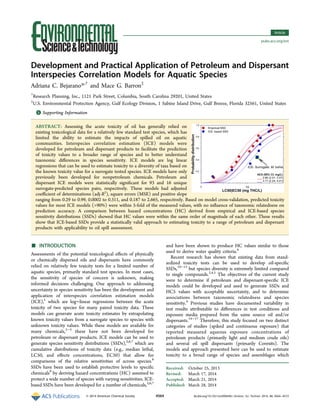
  • 3. protective of 99% or 95% of the species in the SSD (i.e., HC1 and HC5, respectively) were computed from the modeled SSD function. All SSDs and HC values were derived using an approach described elsewhere.25 Briefly, toxicity values were fitted to a log-normal distribution function, and SSDs randomly resampled 2000 times to derive the HC1 and HC5 values and their associated 95% confidence intervals (95% CI). Only SSDs that passed goodness of fit tests (α = 0.01) (the Anderson− Darling for SSDs with >7 species, and the Kolmogorov− Smirnov test statistics) were included in these analyses. SSDs were also generated using empirical data for the same categories of petroleum products and dispersants, as well as using a combination of empirical data and ICE-based toxicity values. SSDs with empirical data were generated by calculating the geometric mean of all toxicity values available for each unique species. The geometric was used because it gives less weight to influential data or potentially outliers, leading to conservative estimates.8 To determine if ICE-based SSDs are a viable alternative to the estimation of SSDs where toxicity data are limiting, ICE-based SSDs were compared to empirically based SSDS using log-likelihood statistics.21 This approach compares the log-likelihood values of individual SSDs (e.g., M. beryllina ICE-based and empirical data) with the fitted SSDs of the combined (pooled) model (e.g., M. beryllina ICE-based plus empirical data), testing the hypothesis (via the chi-square statistic) that these SSDs are derived from the same fitted log- normal curve. The same approach was used to compare ICE- based SSDs pairs. All the analyses above were performed using the R statistical platform (v. 2.13.2).22 ■ RESULTS Model Development and Verification. A total of 93 petroleum ICE models for 29 surrogate species, and 16 dispersant ICE models for seven surrogate species were statistically significant (p-value <0.05 for both, the F-test for the overall fit and the t test for the slope parameter) (SI Tables S1−S3, Figures S2 and S3). Models lacking significance typically had limited paired data (22 petroleum and 5 dispersant ICE models with <5 paired data points) limiting their use in further analyses. The validity of statistically significant models was verified using standard regression diagnostics procedures.20 Visual examination of the standardized residuals of each significant model (Figure 1, left panel) showed that all residuals fell within a horizontal band centered on 0, indicating that the variance of the error term was constant. No obvious outliers were detected (±4 standardized residual values). Diagnostic analyses also indicated that the error term did not depart substantially from a normal distribution (Figure 1, right panel), as the coefficient of determination (R2 ) between residuals and quantiles for petroleum and dispersant ICE models were greater (0.997 and 0.991, respectively) than those of the critical R2 value (0.985) (α = 0.05; n ≥ 100).26 A moderate departure from normality was noted at the end tails of the distributions, particularly for petroleum ICE models (14 data points) but was considered minimal because removal of these data points did not cause major changes in fitted values. In all cases, the absolute change between fitted values with and without potentially influential points ranged from 4 to 11% indicating no disproportional influence on fitted values. Statistically significant models had an adjusted coefficient of determination (adj-R2 ) ranging from 0.29 and 0.99, a Mean Square Error (MSE; a measure of fit) ranging from 0.0002 to 0.311, and a positive slope ranging from 0.187 to 2.665 (SI Tables S2 and S3). Examination of model parameter viability shows that 92% of all intercepts were between −0.75 and 0.75, and that 85% of all slopes were between 0.5 and 1.5. This relatively narrow variability suggests similarities across most models. Notable exceptions, where both the slope and intercept of the same model were outside these ranges included (1) the petroleum ICE models for the surrogate-predicted pairs Calanus sinicus- Paracalanus aculeatus (both copepods species), Cyprinodon variegatus (sheepshead minnow)-A. bahia, and Pontogammarus maeoticus (amphipod)-Calanipeda aquae dulcis (copepod); and (2) the dispersant ICE models for the pairs C. variegatus-A. bahia, A. affinis-H. costata, and A. affinis- Macrocystis pyrifera (giant kelp). In these deviating cases, except pairs involving A. affinis, the predicted species was generally more sensitivity than the surrogate species, but in all cases MSE were small (below 0.16). Figure 1. Diagnostic analyses of homogeneity of variances (left) and normality (right) for petroleum and dispersant ICE models. Environmental Science & Technology Article dx.doi.org/10.1021/es500649v | Environ. Sci. Technol. 2014, 48, 4564−45724566
  • 4. The reliability and predictive power of statistically significant models was further assessed by identifying the MSE cutoff associated with a-priori cross-validation success rates of 85% and 95%,5 assumed to have moderate and high reliabilities, respectively (Figure 2). MSE cutoffs for petroleum and dispersant models were 0.126 and 0.04, respectively. Over half of the petroleum ICE models (54 models) had MSEs ≤0.04, while over 30% (32 models) had MSEs between 0.04 and 0.126. By comparison, dispersant ICE models were equally distributed among MSE cutoffs, suggesting that petroleum ICE models may be more robust. The high cross-validation success rate (a measure of predictive power) was consistent with the agreement between predicted and observed values for both ICE models types (Figure 3). For petroleum ICE models, 98% of the predicted values were within 5-fold difference of the observed data, with most values (92%) being within 2-fold difference of the observed data. There was no influence of taxonomic relatedness on prediction accuracy (p-value >0.05), and mean fold- difference values across taxonomic distances ranged from 1.00 to 1.38 (SI Figure S4). Only 0.5% of predicted values (seven observations) were >10-fold difference from the observed values. These outliers occurred only in the M. beryllina- A. bahia (taxonomic distance = 6), Daphnia magna (water flea)- Artemia salina (brine shrimp) (taxonomic distance=4), and A. bahia- M. beryllina surrogate- predicted pairs (3, 3, and 1 observations, respectively). For dispersant ICE models, 99% of the predicted values were within 5-fold difference of the observed data, with most values (88%) being within 2-fold of the observed data. There was no influence of taxonomic relatedness on prediction accuracy (p-value >0.05), and mean fold-difference values were 1.29 and 1.14 for taxonomic distances 6 and 7, respectively. The largest fold difference of 7 occurred in the A. bahia- M. beryllina surrogate- predicted pair. Practical Application of ICE Models. Toxicity data for several petroleum products from an analysis independent of the research presented here10 were used to verify the applicability of ICE models. Two sets of SSD were developed using ICE models for A. bahia and M. beryllina as the surrogate species, with input surrogate concentrations from Barron et al.10 The first set of SSDs used all ICE models regardless of their reliability, while the second set used only ICE models with MSE <0.12. Statistical comparison of SSDs via (using the log- likelihood),21 showed that these two types of SSDs for several petroleum products and for both surrogate species, were not significantly different from each other (p-value >0.05). This indicates that exclusion of the least reliable models did not influence the shape of the SSD. No statistically significant differences were also found between A. bahia and M. beryllina ICE-based SSDs (p-value >0.05), or between either of these two ICE-based SSDs and empirical SSDs10 (p-value >0.05; Figure 4). Estimated petroleum hydrocarbon HC5s from ICE- based SSDs were in general agreement with those derived from SSDs using empirical data10 (SI Table S5), though values from M. beryllina as the surrogate were generally larger (up to a 6 fold larger) than those calculated from empirical data. A second verification approach utilized empirical toxicity data for physically and chemically dispersed combined from constant and spiked exposures, as well as toxicity data for Corexit 9500 and Corexit 9727,18 which were used to generate SSDs (Figure 5). The selection of these data was driven by the fact that these SSDs shared data for two surrogate species: H. costata and A. bahia. SSDs were derived using all ICE models Figure 2. Assessment of model reliability based on the relationship between model mean square error (MSE) and cross-validation success rate for both, petroleum and dispersant ICE models. Figure 3. Comparison of observed and ICE-predicted toxicity values for petroleum hydrocarbons and dispersants. The solid line represents the 1:1 line (equal toxicity), while the dotted lines represent a 5-fold difference between these values. Bar chart on the right, display the fold-difference between observed and ICE-predicted toxicity values. Environmental Science & Technology Article dx.doi.org/10.1021/es500649v | Environ. Sci. Technol. 2014, 48, 4564−45724567
  • 5. for these surrogate species regardless of model reliability. Because there were insufficient paired surrogate-predicted ICE models for the same surrogate species to generate SSDs for dispersants (five species minimum), predicted ICE model concentrations were combined for H. costata and A. bahia. Curve comparison of empirically and ICE-based SSDs, using log-likelihood, showed no statistically significant differences between A. bahia and H. costata ICE-based SSDs (p-value >0.05), or between either of these two ICE-based SSDs and empirical SSDs10,18 (p-value >0.05), with one exception: the H. costata ICE-based SSDs and the empirical SSDs18 for constant exposures to dispersed oil (p-value = 0.01; Figure 5). In most cases, ICE-based models with H. costata and A. bahia as surrogates, produced smaller HC5s indicative of a slight model bias toward overprotection of aquatic species. In all cases, HC5s from ICE-based SSDs were within the same order of magnitude as HC5s from empirical SSDs. HC5s for Corexit 9500 and Corexit 9727 from ICE-based SSDs were also similar to those reported by Barron et al.10 Hazard concentrations (96 h HC1 and HC5) were estimated for fresh petroleum and dispersant products for which data, on the basis of measured concentrations, were available from constant static and spiked flow-through exposures (Table 1). These hazard concentrations were estimated using ICE-based SSD with models from each of two surrogate species (A. bahia and M. beryllina). An additional set of SSDs was also constructed by combining all available empirical data plus Figure 4. Comparison between species sensitivity distribution (SSD) curves for all petroleum products from Barron et al.10 (dashed line), and SSDs derived using all ICE models, regardless of their reliability, with A. bahia (black dots and lines) and M. beryllina (blue dots and lines) as the surrogate species. These curves are not significantly different (p-value >0.05) from each other. Figure 5. Comparison between physically and chemically dispersed oil (top), and dispersant (bottom) species sensitivity distribution (SSD) using empirical18 and ICE-based models (red dots and lines; red dashed line from Barron et al.10 for dispersants only). SSDs using empirical data for dispersed oil were developed for constant and spiked exposures separately. SSDs were derived using all ICE models regardless of their reliability with A. bahia (black dots and lines) and H. costata (blue dots and lines) as surrogate species, combining models for these two species for dispersant SSDs (black lines). Within panels, SSDs are not significantly different (p-value > 0.05) from each other, except for the comparison of H. costata ICE-based SSDs and the empirical SSDs for constant exposures to dispersed oil (p-value = 0.01; top left). Environmental Science & Technology Article dx.doi.org/10.1021/es500649v | Environ. Sci. Technol. 2014, 48, 4564−45724568
  • 6. ICE toxicity values for one or more surrogate species (A. bahia, H. costata, M. beryllina and A. affinis), keeping the smallest predicted value for each unique predicted- species (SI Figure S5). Starting concentrations for surrogate species were those of studies reporting measured toxicity data,14,15,27−37 and excluded from model development. HC1s and HC5s for seven fresh oils and by oil category ranged from 0.13 mg THC/L to 3.72 mg THC/L, and from 0.16 to 4.92 mg THC/L, respectively. Venezuelan crude oil had the lowest HC values (more toxic), while Alaska North Slope oil had the highest values (less toxic). HC values from ICE-based SSDs with A. bahia as the surrogate species were similar to those with M. beryllina, and were generally within the same order of magnitude of each other. HC values from SSDs that combined empirical data and predicted toxicity values from one or more surrogate species were also similar to those derived with either A. bahia or M. beryllina. In all cases, spiked flow-through exposures produced HC values up to 12 times greater than HC values from static exposures, with Venezuelan and Alaska North Slope crude oil having the largest and smallest differences, respectively, between these exposure types. SSDs using A. bahia or M. beryllina as surrogate species, and SSDs with empirical plus ICE Table 1. Estimated HC1 and HC5 Petroleum Hydrocarbon (THC) Concentrations (mg/L) for Specific Petroleum and Dispersant Products and Exposure Regimesa petroleum/dispersant product experimental conditions surrogate: A. bahia HC1 (first row) | HC5 (second row) (95% CI) surrogate: M. beryllina HC1 (first row) | HC5 (second row) (95% CI) empirical+ ICE-predicted HC1 (first row) | HC5 (second row) (95% CI) Alaska North constant static 0.55 (0.30−0.92) 3.03 (1.96−4.55) 0.45 (0.24−0.77) Slope 0.69 (0.44−1.02) 3.97 (2.93−5.35) 0.63 (0.37−0.99) flow-through 1.03 (0.61−1.60) 3.72 (2.44−5.63) 1.27 (0.75−2.06) 1.32 (0.93−1.86) 4.92 (3.69−6.57) 1.72 (1.09−2.58) Arabian flow-through NA 0.59 (0.34−0.95) NA Medium NA 0.71 (0.49−1.00) NA Forties constant static 0.15 (0.07−0.28) 0.14 (0.06−0.29) 0.17 (0.07−0.34) 0.18 (0.10−0.29) 0.16 (0.08−0.26) 0.18 (0.09−0.36) flow-through 2.32 (1.41−3.66) 2.10 (1.36−3.16) 1.76 (1.05−2.72) 3.06 (2.11−4.29) 2.70 (1.98−3.62) 2.28 (1.50−3.35) Kuwait constant static 0.23 (0.11−0.41) 0.21 (0.10−0.37) 0.23 (0.12−0.41) 0.28 (0.17−0.42) 0.23 (0.14−0.37) 0.26 (0.15−0.43) flow-through 2.62 (1.58−4.29) 1.56 (1.01−2.31) 1.26 (0.77−1.9) 3.49 (2.43−4.95) 1.97 (1.45−2.61) 1.57 (1.05−2.23) Prudhoe Bay constant static NA 1.94 (1.24−2.84) NA NA 2.48 (1.82−3.31) NA flow-through 2.40 (1.40−3.90) 3.11 (2.01−4.68) 3.54 (2.24−5.41) 3.19 (2.21−4.50) 4.09 (3.03−5.40) 4.52 (3.14−6.42) South constant static 0.92 (0.51−1.49) 1.27 (0.80−1.94) 0.75 (0.43−1.20) Louisiana 1.15 (0.76−1.68) 1.58 (1.16−2.10) 0.97 (0.63−1.49) Venezuelan constant static 0.13 (0.06−0.24) 0.19 (0.09−0.36) 0.16 (0.07−0.31) 0.16 (0.09−0.25) 0.21 (0.12−0.35) 0.18 (0.09−0.32) flow-through 2.12 (1.27−3.38) 0.29 (0.14−0.50) 0.36 (0.19−0.61) 2.78 (1.94−3.93) 0.33 (0.20−0.50) 0.42 (0.25−0.66) Light crudesb constant static 0.19 (0.09−0.35) 0.44 (0.24−0.74) 0.22 (0.11−0.39) 0.24 (0.13−0.4) 0.53 (0.31−0.82) 0.29 (0.16−0.47) flow-through 0.84 (0.45−1.44) 0.64 (0.37−1) 0.36 (0.17−0.66) 1.07 (0.61−1.74) 0.78 (0.48−1.2) 0.47 (0.24−0.82) Medium constant static 0.62 (0.41−0.89) 1.21 (0.74−1.88) 0.27 (0.12−0.49) crudesc 0.71 (0.50−0.98) 1.50 (0.98−2.21) 0.35 (0.17−0.62) flow-through 1.74 (1.04−2.85) 1.72 (1.09−2.63) 2.35 (1.52−3.54) 2.25 (1.44−3.55) 2.20 (1.51−3.12) 2.98 (2.08−4.14) Corexit 7664 flow-through NA NA 375 (182−744) 789 (478−1145) Corexit 9500 constant static NA NA 2.24 (1.25−3.73) 3.33 (2.15−5.13) flow-through NA NA 27 (16−42) 40 (27−60) Corexit 9527 constant static NA NA 1.09 (0.62−1.80) 1.62 (1.02−2.49) flow-through NA NA 5.51 (3.44−8.60) 7.65 (5.27−11.02) a HC Values were generated from ICE-based SSDs using surrogate-predicted ICE Models with at least five pairs per unique surrogate, as well as by combining empirical and ICE predicted toxicity data from one or more surrogate species. Known surrogate concentrations include 96 h THC toxicity data from physically dispersed fresh oil and fresh oil chemically dispersed with Corexit 9500, except for Kuwait Oil, which was chemically dispersed with Corexit 9527. Surrogate toxicity data are the geometric mean of all measured values for the same species.14,15,27−37 NA, data not available. b Forties + South Louisiana + Venezuelan. c Alaska North Slope + Arabian Medium + Kuwait + Prudhoe Bay. Environmental Science & Technology Article dx.doi.org/10.1021/es500649v | Environ. Sci. Technol. 2014, 48, 4564−45724569
  • 7. toxicity values were not statistically different (p-value > 0.05) within petroleum products and by experimental condition. While there were insufficient dispersant ICE models for A. bahia or M. beryllina as surrogate species to produce ICE-based SSDs, combined data from empirical and ICE toxicity values allowed the estimation HC values for three dispersants. ■ DISCUSSION One of the greatest challenges in evaluating potential impacts to aquatic communities during oil spills and impact assessment continues to be uncertainties in species sensitivity. The Deepwater Horizon oil spill further highlighted the need to understand the sensitivity of the diversity of aquatic species in the deep ocean, pelagic and coastal areas with generally limited existing toxicity data.38 The current study provides both petroleum and dispersant-specific toxicity estimation models that can be applied to a broad range of aquatic species assemblages using a SSD-based approach. The practical use of existing oil toxicity data has been limited by the general lack of standardized laboratory practices, including differences in media preparation.13,14,39,40 While these issues may have added uncertainty to the development of petroleum and dispersant ICE models, emphasis was placed on rigorously standardizing data selection with the sole intent of reducing the uncertainty introduced by differences in experimental procedures across studies. As a result, and despite inherent limitations with existing data, all statistically significant ICE models had a relatively small MSE (range 0.0002−0.311), indicative of a robust model fit. As indicated elsewhere,6 and applicable here, these robust ICE model relationships suggest that the same mechanisms of action for each species pair may be at play. Furthermore, MSE values associated with 85% and 95% cross-validation success rates of ICE models were smaller (0.126 and 0.04, respectively) than MSE values associated with the same cutoffs (0.22 and 0.15, respectively) for ICE models with wildlife species.5 In addition, predicted values from ICE models were generally within 5-fold difference of the observed data, with most models being within 2-fold of the observed data. These predicted-observed differences are well within the fold difference commonly found across laboratories (fold difference of 3)41 during optimal interlaboratory comparisons with the same species. Taxonomic relatedness has been previously shown to influence model fit and reliability of ICE models developed from chemicals with mixed modes of action.4,5 In contrast, petroleum and dispersant-specific ICE models showed no influence of taxonomic distance on model accuracy. These results suggest that ICE models developed with chemicals with a common nonspecific mode of chemical action such as narcosis can be used to predict toxicity across a broad range of taxa, and can help improve predictions over ICE models from with mixed modes of action. While SSDs have been used in the field of aquatic toxicology and integrated into the regulatory framework,42 their use in oil spill research has been limited.10−12 SSDs and derived benchmarks can be used to protect untested species under the assumption that their sensitivity is within the range of sensitivities captured by the species in the SSD. Although SSDs cannot replace toxicity testing, they can provide additional information when the costs of toxicity testing are prohibitive or species-specific testing is restricted or not feasible (e.g., endangered, rare, deepwater species). Furthermore, both empiric and ICE-based SSDs can help inform resource managers in their assessment of potential acute effects associated with petroleum or dispersant products, particularly when data are limited. Moreover, data from concurrent toxicity testing of rarely investigated taxa (e.g., corals, pelagic fish) and a surrogate species for which ICE models are available (e.g., A. bahia or M. beryllina), can be used to construct an ICE-based SSD allowing for the placement in the curve of the species for which little toxicity data, facilitating comparisons of relative sensitivities. As demonstrated here, ICE models could be used to augment estimates of benchmark concentrations from spiked flow-through exposures that may be more applicable to short- duration oil spills, and for which toxicity data are less available in the scientific literature.13 As shown here and elsewhere,2,6,7 ICE-based SSDs can produce HC5 values similar to those generated from empirical SSDs, adding reliability to the use of ICE models to augment toxicity data. Here, HC5s from ICE- based SSDs for petroleum and Corexit dispersants were within 1 order of magnitude HC5s from SSDs with empirical data.10,18 While previous studies have recommended between 7 and 15 species to develop reliable SSDs and associated benchmarks,2,7 the minimum number of species used here was 5. As a result, petroleum ICE-based SSDs could only be developed for 9 surrogate species (including A. bahia and M. beryllina), or by combining data for at least two species as demonstrated with the dispersant ICE-based SSDs. While A. bahia generally appears to be more sensitivity than M. beryllina (as shown here and elsewhere10 ), SSDs from ICE models with M. beryllina as the surrogate species did not result in significantly larger HC values. Consequently, the surrogate set of models that leads to smaller HC values may be preferred, particularly when protection of especially sensitive species is a concern, or when there are concerns about species in specific microhabitat (e.g., sheltered salt marshes, mangroves or tidal flats) within coastal ecosystems. One of the limitations of the current study is that, because of the nature of the existing toxicity data, models were developed under the assumption that petroleum hydrocarbons represent a single compound with a predominant mode of toxicity (nonpolar narcosis). In reality, petroleum hydrocarbons are a complex mixture of chemicals with more than one mode of toxicity (narcosis, receptor-mediated). Because compounds in these mixtures have different chemical properties and affinities for lipids, it is widely recognized that their composition determine their overall toxicity.43−45 This limitation, however, could be overcome by using quantitative structure activity relationships (QSARs),2 which are relationships based on chemical structure. QSAR toxicity data can provide surrogate values for the development of hydrocarbon-specific ICE models,2 or could be used to develop QSAR surrogate- predicted species ICE models.46 Future refinements of ICE models are dependent upon greater availability of detailed analytical chemistry results (e.g., individual PAH analytes), which are currently lacking in most petroleum and dispersant toxicity data sources.13 In this study petroleum and dispersant ICE models were developed and used to generate ICE-based SSDs. While the development of ICE models was limited by the availability of toxicity data meeting the rigorous standardization criteria, the information presented here could facilitate assessments of the potential toxicological consequences oil and dispersants to aquatic communities, aid in the estimation of concentration associated with low or no effects, and allow for comparisons of the relative sensitivity across test species. ICE-based SSDs could also be used in conjunction with environmental Environmental Science & Technology Article dx.doi.org/10.1021/es500649v | Environ. Sci. Technol. 2014, 48, 4564−45724570
  • 8. concentrations from fate models or environmental monitoring to help characterize, via joint probability distribution curves, the fraction of potentially affected species or the magnitude of adverse effects to aquatic communities.8 The inclusion of additional paired-empirical data for a wider number of species, particularly for sensitive life stages, may allow for further application of ICE models in damage assessments so as to allow comparisons across communities (e.g., epibenthic vs benthic effects assessments) and habitats (e.g., tidal flats vs marshes). While model verification showed promising results, additional toxicity data could help improve existing ICE models and facilitate the development of additional ones. Of special interest is the inclusion of paired standard test-sensitive or rare species toxicity data, which is essential to refine petroleum and dispersant benchmark concentrations protective of the most sensitive or untested species. ■ ASSOCIATED CONTENT *S Supporting Information Additional information related to ICE models is available in Supporting Information 1. This information includes a complete list of references of the original sources, One table containing scientific and common names, two tables containing statistically significant ICE model parameters, 1 Table comparing empirical and ICE based HC5s, 1 Figure of the model building scheme, two figures of the fitted models, one figure on taxonomic relatedness, and one figure with representative SSDs. Supporting Information 2 contains core data used in the development of ICE models. This material is available free of charge via the Internet at http://pubs.acs.org. ■ AUTHOR INFORMATION Corresponding Author *Phone: +1 803 254 0278; fax: + 1 803 254 6445; e-mail: abejarano@researchplanning.com. Notes The authors declare no competing financial interest. ■ ACKNOWLEDGMENTS Special thanks to C. Jackson and S. Raimondo (U.S. EPA) for comments to an earlier version of this manuscript. This research was made possible by a grant from NOAA and the University of New Hampshire’s Coastal Response Research Center (Contract No. 13-034) to Research Planning, Inc. None of these results have been reviewed by CRRC and no endorsement should be inferred. The views expressed in this article are those of the authors and do not necessarily reflect the views or policies of the U.S. EPA. This publication does not constitute an endorsement of any commercial product. ■ ABBREVIATIONS adj-R2 adjusted coefficient of determination HC1 and HC5 1st and fifth percentile hazard concentrations ICE interspecies correlation estimation LC50 and EC50 median lethal and effects concentrations, respectively MSE mean square error SSD species sensitivity distributions THC total hydrocarbon content ■ REFERENCES (1) Asfaw, A., Ellersieck, M. R., Mayer, F. L. Interspecies Correlation Estimations (ICE) for Acute Toxicity to Aquatic Organisms and Wildlife. II. User Manual and Software, EPA/600/R-03/106; United States Environmental Protection Agency: Washington, DC, 2003. (2) Dyer, S. D.; Versteeg, D. J.; Belanger, S. E.; Chaney, J. G.; Mayer, F. L. Interspecies correlation estimates predict protective environ- mental concentrations. Environ. Sci. Technol. 2006, 40 (9), 3102−3111. (3) Golsteijn, L.; Hendriks, H. W.; van Zelm, R.; Ragas, A. M.; Huijbregts, M. A. Do interspecies correlation estimations increase the reliability of toxicity estimates for wildlife? Ecotoxicol. Environ. Saf. 2012, 80, 238−243. (4) Raimondo, S.; Jackson, C. R.; Barron, M. G. Influence of taxonomic relatedness and chemical mode of action in acute interspecies estimation models for aquatic species. Environ. Sci. Technol. 2010, 44 (19), 7711−7716. (5) Raimondo, S.; Mineau, P.; Barron, M. Estimation of chemical toxicity to wildlife species using interspecies correlation models. Environ. Sci. Technol. 2007, 41 (16), 5888−5894. (6) Dyer, S. D.; Versteeg, D. J.; Belanger, S. E.; Chaney, J. G.; Raimondo, S.; Barron, M. G. Comparison of species sensitivity distributions derived from interspecies correlation models to distributions used to derive water quality criteria. Environ. Sci. Technol. 2008, 42 (8), 3076−3083. (7) Awkerman, J. A.; Raimondo, S.; Barron, M. G. Development of species sensitivity distributions for wildlife using interspecies toxicity correlation models. Environ. Sci. Technol. 2008, 42 (9), 3447−3452. (8) Posthuma, L.; Suter II, G. W.; Traas, T. P. Species Sensitivity Distributions in Ecotoxicology; Lewis: Boca Raton, FL, 2002. (9) De Zwart, D., Observed regularities in species sensitivity distributions for aquatic species. In Species Sensitivity Distributions in Ecotoxicology; Posthuma, L., Suter, G. W., Traas, T. P., Ed. Lewis Publishers: Boca Raton, FL, 2002; pp 133−154. (10) Barron, M. G.; Hemmer, M. J.; Jackson, C. R. Development of aquatic toxicity benchmarks for oil products using species sensitivity distributions. Integr. Environ. Assess. Manage. 2013, 9 (4), 610−615. (11) Bejarano, A. C.; Levine, E.; Mearns, A. Effectiveness and potential ecological effects of offshore surface dispersant use during the Deepwater Horizon oil spill: A retrospective analysis of monitoring data. Environ. Monit. Assess. 2013, 185, 10281−10295. (12) de Hoop, L.; Schipper, A. M.; Leuven, R. S.; Huijbregts, M. A.; Olsen, G. H.; Smit, M. G.; Hendriks, A. J. Sensitivity of polar and temperate marine organisms to oil components. Environ. Sci. Technol. 2011, 45 (20), 9017−9023. (13) Bejarano A. C.; Clark J. R.; Coelho, J. M., Issues and challenges with oil toxicity data and implications for their use in decision making: A quantitative review. In Environ. Toxicol. Chem. DOI: 10.1002/ etc.2501, 2014. (14) Aurand, D.; Coelho, G. Cooperative Aquatic Toxicity Testing of Dispersed Oil and the “Chemical Response to Oil Spills: Ecological Effects Research Forum (CROSERF)”. Technical Report.; EM&A Inc.: Lusby, MD, 2005; p 79. (15) Clark, J. R.; Bragin, G. E.; Febbo, R.; Letinski, D. J. In Toxicity of Physically and Chemically Dispersed Oils under Continuous and Environmentally Realistic Exposure Conditions: Applicability to Dispersant Use Decisions in Spill Response Planning, Proceedings of the 2001 International Oil spill Conference; American Petroleum Institute: Tampa, FL, March 26−29, 2001; pp 1249−1255. (16) Singer, M.; Smalheer, D.; Tjeerdema, R.; Martin, M. Toxicity of an oil dispersant to the early life stages of four California marine species. Environ. Toxicol. Chem. 1990, 9 (11), 1387−1395. (17) Singer, M. M.; George, S.; Jacobson, S.; Lee, I.; Tjeerdema, R. S.; Sowby, M. L. Comparative toxicity of Corexit ® 7664 to the early life stages of four marine species. Arch. Environ. Contam. Toxicol. 1994, 27 (1), 130−136. (18) Bejarano, A. C.; Chu, V.; Farr, J.; Dahlin, J., Development and application of DTox: A quantitative database of the toxicological effects of dispersants and chemically dispersed oil. In Proceedings of the Environmental Science & Technology Article dx.doi.org/10.1021/es500649v | Environ. Sci. Technol. 2014, 48, 4564−45724571
  • 9. 2014 International Oil Spill Conference, American Petroleum Institute: Savanah, GA, 2014, in press. (19) USEPA, ECOTOX. Release 4.0. Ecotoxicology Database; US Environmental Protection Agency: Duluth, MN, 2012. www.epa.gov/ ecotox. (20) Neter, J.; Wasserman, W.; Kutner, M. H., Applied Linear Statistical Models: Regression, Analysis of Variance, And Experimental Designs; McGraw-Hill Higher Education: Boston, MA, 1990. (21) Piegorsch, W. W.; Bailer, A. J., Statistics for Environmental Biology and Toxicology; Chapman & Hall: London, UK., 1997. (22) R: A Language and Environment for Statistical Computing,Version 2.13.2011-09-30; R Development Core Team: Vienna, Austria, 2011. (23) Canty, A.; Ripley, B. boot: Bootstrap R (S-Plus) Functions, R package version 1.3-9, 2013. (24) Davison, A. C.; Hinkley, D. V., Bootstrap Methods and Their Applications; Cambridge University Press: Cambridge, 1997. (25) Bejarano, A. C.; Farr, J. K. Development of short acute exposure hazard estimates: A tool for assessing the effects of chemical spills in aquatic environments. Environ. Toxicol. Chem. 2013, 32 (8), 1918− 1927. (26) Looney, S. W.; Gulledge, T. R., Jr Use of the correlation coefficient with normal probability plots. Am. Stat. 1985, 39 (1), 75− 79. (27) Bragin, G.; Clark, J.; Pace, C. Comparison of Physically and Chemically Dispersed Crude Oil Toxicity to Both Regional and National Test Species under Continuous and Spiked Exposure Scenarios, MSRC Technical Report Series 94-015; Marine Spill Response Corporation: Washington, DC, 1994; pp 1−45. (28) Bragin, G. E.; Clark, J. R. Chemically Dispersed Crude Oils: Toxicity to Regional and National Test Species under Constant and Spiked Exposures; Marine Spill Response Corporation: Washington DC, 1995; pp 1−44. (29) Hemmer, M. J.; Barron, M. G.; Greene, R. M. Comparative toxicity of eight oil dispersants, Louisiana sweet crude oil (LSC), and chemically dispersed LSC to two aquatic test species. Environ. Toxicol. Chem. 2011, 30 (10), 2244−2252. (30) Pace, C. B.; Clark, J. R.; Bragin, G. E. In Comparing Crude Oil Toxicity under Standard and Environmentally Realistic Exposures, Proceedings of the 1995 International Oil Spill Conference; American Petroleum Institute: Washington, DC, February 27 to March 2, 1995, 1995; pp 1003−1004. (31) Perkins, R. A.; Rhoton, S.; Behr-Andres, C. Toxicity of dispersed and undispersed, fresh and weathered oil to larvae of a cold-water species, Tanner crab (C. bairdi), and standard warm-water test species. Cold Reg. Sci. Technol. 2003, 36 (1), 129−140. (32) Perkins, R. A.; Rhoton, S.; Behr-Andres, C. Comparative marine toxicity testing: A cold-water species and standard warm-water test species exposed to crude oil and dispersant. Cold Reg. Sci. Technol. 2005, 42 (3), 226−236. (33) Rhoton, S. Acute Toxicity of the Oil Dispersant Corexit 9500, and Fresh and Weathered Alaska North Slope Crude Oil to the Alaskan Tanner Crab (C. bairdi), Two Standard Test Species, and V. fischeri (Microtox Assay). MSc Thesis, Institute of Northern Engineering, University of Alaska: Fairbanks, AK 2000. (34) Wetzel, D.; Van Fleet, E. S. In Cooperative Studies on the Toxicity of Dispersants and Dispersed Oil to Marine Organisms: A 3-Year Florida Study, Proceedings of the 2001 International Oil spill Conference; American Petroleum Institute: Tampa, FL, March 26−29, 2001; pp 1237−1241. (35) Gardiner, W.; Word, J.; Word, J.; Perkins, R.; McFarlin, K.; Hester, B.; Word, L.; Ray, C. The acute toxicity of chemically and physically dispersed crude oil to key arctic species under arctic conditions during the open water season. Environ. Toxicol. Chem. 2013, 32 (10), 2284−2300. (36) Singer, M.; George, S.; Lee, I.; Jacobson, S.; Weetman, L.; Blondina, G.; Tjeerdema, R.; Aurand, D.; Sowby, M. Effects of dispersant treatment on the acute aquatic toxicity of petroleum hydrocarbons. Arch. Environ. Contam. Toxicol. 1998, 34 (2), 177−187. (37) Singer, M. M.; Jacobson, S.; Tjeerdema, R. S.; Sowby, M. In Acute Effects of Fresh versus Weathered Oil to Marine Organisms: California Findings, Proceedings of the 2001 International Oil Spill Conference; American Petroleum Institute, Tampa, FL, USA, March 26−29, 2001; pp 1263−1268. (38) Carriger, J. F.; Barron, M. G., Minimizing risks from spilled oil to ecosystem services using influence diagrams: The Deepwater Horizon spill response. Environ. Sci. Technol. 45, (18), 7631-7639. (39) Coelho, G.; Clark, J.; Aurand, D. Toxicity testing of dispersed oil requires adherence to standardized protocols to assess potential real world effects. Environ. Pollut. 2013, 177, 185−188. (40) Singer, M.; Tjeerdema, R.; Aurand, D.; Clark, J.; Sergy, G.; Sowby, M. In CROSERF: Toward a Standardization of Oil Spill Cleanup Agent Ecological Effects Research, Arctic and marine oil spill program technical seminar, 1995; Ministry of Supply and Services: Canada, 1995; pp 1263−1270. (41) Rand, G.; Wells, P.; McCarty, L. Chapter 1. Introduction to Aquatic Toxicology. In Fundamentals of Aquatic Toxicology Effects, Environmental Fate, And Risk Assessment; Rand, G., Ed.; Taylor and Francis Publishers: North Palm Beach, FL, 1995; pp 3−67. (42) Barron, M. G.; Wharton, S. R. Survey of methodologies for developing media screening values for ecological risk assessment. Integr. Environ. Assess. Manage. 2005, 1 (4), 320−332. (43) Di Toro, D. M.; McGrath, J. A.; Hansen, D. J. Technical basis for narcotic chemicals and polycyclic aromatic hydrocarbon criteria. I. Water and tissue. Environ. Toxicol. Chem. 2000, 19 (8), 1951−1970. (44) Di Toro, D. M.; McGrath, J. A.; Stubblefield, W. A. Predicting the toxicity of neat and weathered crude oil: Toxic potential and the toxicity of saturated mixtures. Environ. Toxicol. Chem. 2007, 26 (1), 24−36. (45) USEPA Procedures for the Derivation of Equilibrium Partitioning Sediment Benchmarks (ESBs) for the Protection of Benthic Organisms: PAH Mixtures. EPA-600-R-02-013. http://www. epa.gov/nheerl/download_files/publications/PAHESB.pdf (accessed 8 March 2013). (46) Chicu, S.; Putz, M. Köln-Timişoara Molecular activity combined models toward interspecies toxicity assessment. Int. J. Mol. Sci. 2009, 10 (10), 4474−4497. Environmental Science & Technology Article dx.doi.org/10.1021/es500649v | Environ. Sci. Technol. 2014, 48, 4564−45724572