finite impulse response

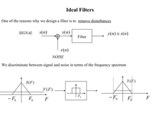
1. Ideal Filters
One of the reasons why we design a filter is to remove disturbances
⊕
)(ns
)(nv
)(nx )()( nsny ≅
Filter
SIGNAL
NOISE
We discriminate between signal and noise in terms of the frequency spectrum
F
)(FS
)(FV
0F0F− 0F
F
)(FY
0F0F−

2. Conditions for Non-Distortion
Problem: ideally we do not want the filter to distort the signal we want to recover.
IDEAL
FILTER
)()( tstx = )()( TtAsty −= Same shape as s(t),
just scaled and
delayed.
0 200 400 600 800 1000
-2
-1.5
-1
-0.5
0
0.5
1
1.5
2
0 200 400 600 800 1000
-2
-1.5
-1
-0.5
0
0.5
1
1.5
2
Consequence on the Frequency Response:



=
−
otherwise
passbandtheinisFifAe
FH
FTj
0
)(
2π
F
F
|)(| FH
)(FH∠
constant
linear

3. For real time implementation we also want the filter to be causal, ie.
0for0)( <= nnh
•
•
• •
•
•
•
••
h n( )
n
•
 since
∑
+∞
=
−=
0
)()()(
k
knxkhny 
onlyspast value
FACT (Bad News!): by the Paley-Wiener Theorem, if h(n) is causal and with finite energy,
∫
+
−
∞+<
π
π
ωω dH )(ln
ie cannot be zero on an interval, therefore it cannot be ideal.)(ωH
∫ +∞=⇒−∞== ωωω dHH )(log)0log()(log
1ω 2ω 1ω
2ω

4. Characteristics of Non Ideal Digital Filters
ω
|)(| ωH
pω
IDEAL
Positive freq. only
NON IDEAL

5. Two Classes of Digital Filters:
a) Finite Impulse Response (FIR), non recursive, of the form
)()(...)1()1()()0()( NnxNhnxhnxhny −++−+=
With N being the order of the filter.
Advantages: always stable, the phase can be made exactly linear, we can approximate any
filter we want;
Disadvantages: we need a lot of coefficients (N large) for good performance;
b) Infinite Impulse Response (IIR), recursive, of the form
)(...)1()()(...)1()( 101 NnxbnxbnxbNnyanyany NN −++−+=−++−+
Advantages: very selective with a few coefficients;
Disadvantages: non necessarily stable, non linear phase.

6. Finite Impulse Response (FIR) Filters
Definition: a filter whose impulse response has finite duration.
•
•
• •
•
•
•
••• • •
h n( )
n
h n( )
x n( ) y n( )
h n( ) = 0h n( ) = 0
•••••• •••••

7. Problem: Given a desired Frequency Response of the filter, determine the impulse
response .
Hd ( )ω
h n( )
Recall: we relate the Frequency Response and the Impulse Response by the DTFT:
{ } ∑
+∞
−∞=
−
==
n
nj
ddd enhnhDTFTH ω
ω )()()(
{ } ∫
+
−
==
π
π
ω
ωω
π
ω deHHIDTFTnh nj
ddd )(
2
1
)()(
Example: Ideal Low Pass Filter
+π−π +ωc−ωc
Hd ( )ω
A
ω
( ) c
sin1
( ) sinc
2
c
c
cj n c
d
n
h n Ae d A A n
n
ω
ω
ω
ω ω ω
ω
π π π π
+
−
 
= = =  ÷
 
∫
)(nhd
n
ω
π
c=
4
DTFT

8. Notice two facts:
• the filter is not causal, i.e. the impulse response h(n) is non zero for n<0;
• the impulse response has infinite duration.
This is not just a coincidence. In general the following can be shown:
If a filter is causal then
• the frequency response cannot be zero on an interval;
• magnitude and phase are not independent, i.e. they cannot be specified arbitrarily
⇒•
•
•
•
•
••
h n( )
••
h n( ) = 0
H( )ω
H( )ω = 0
As a consequence: an ideal filter cannot be causal.

9. Problem: we want to determine a causal Finite Impulse Response (FIR) approximation of the
ideal filter.
We do this by
a) Windowing
-100 -50 0 50 100
-0.1
-0.05
0
0.05
0.1
0.15
0.2
0.25
-100 -50 0 50 100
-0.1
-0.05
0
0.05
0.1
0.15
0.2
0.25
-100 -50 0 50 100
-0.1
-0.05
0
0.05
0.1
0.15
0.2
0.25
-100 -50 0 50 100
0
0.2
0.4
0.6
0.8
1
1.2
1.4
1.6
1.8
2
-100 -50 0 50 100
0
0.2
0.4
0.6
0.8
1
1.2
1.4
1.6
1.8
2
)(nhd
)(nhw
×
=
=
rectangular window
hamming window )(nhw
infinite impulse response
(ideal)
finite impulse response
L− L
L− L
L− L
L− L

10. b) Shifting in time, to make it causal:
-100 -50 0 50 100
-0.1
-0.05
0
0.05
0.1
0.15
0.2
0.25
-100 -50 0 50 100
-0.1
-0.05
0
0.05
0.1
0.15
0.2
0.25
)(nhw
)()( Lnhnh w −=

11. Effects of windowing and shifting on the frequency response of the filter:
a) Windowing: since then)()()( nwnhnh dw = )(*)(
2
1
)( ωω
π
ω WHH dw =
ωcωcω−
)(ωdH
0 0.5 1 1.5 2 2.5 3
-120
-100
-80
-60
-40
-20
0
20
0 0.5 1 1.5 2 2.5 3
-120
-100
-80
-60
-40
-20
0
20
0 0.5 1 1.5 2 2.5 3
-120
-100
-80
-60
-40
-20
0
20
40
0 0.5 1 1.5 2 2.5 3
-120
-100
-80
-60
-40
-20
0
20
40
*
*
=
|)(| ωW |)(| ωwHrectangular window
hamming window
0 0.5 1 1.5 2 2.5 3
-120
-100
-80
-60
-40
-20
0
20
=

12. 0 0.5 1 1.5 2 2.5 3
-120
-100
-80
-60
-40
-20
0
20
ω∆
attenuation
For different windows we have different values of the transition region and the attenuation in the
stopband:
transition
region
Rectangular -13dB
Bartlett -27dB
Hanning -32dB
Hamming -43dB
Blackman -58dB
N/4π
N/8π
N/8π
N/8π
16 / Nπ
ω∆ nattenuatio
-100 -50 0 50 100
-0.1
-0.05
0
0.05
0.1
0.15
0.2
0.25
L− L
12 += LN
)(nhw
n
with

13. Effect of windowing and shifting on the frequency response:
b) shifting: since then)()( Lnhnh w −=
Lj
w eHH ω
ωω −
= )()(
Therefore
phase.inshift)(H)H(
magnitude,on theeffectno)()(
w L
HH w
ωωω
ωω
−∠=∠
=
See what is ).(ωwH∠
For a Low Pass Filter we can verify the symmetry Then).()( nhnh ww −=
)cos()(2)0()()(
1
nnhhenhH
n
ww
nj
n
ww ωω ω
∑∑
+∞
=
−
+∞
−∞=
+==
real for all . Thenω



=∠
otherwise,'
passband;in the0
)(
caretdon
Hw ω

14. The phase of FIR low pass filter:
passband;in the)( LH ωω −=∠
Which shows that it is a Linear Phase Filter.
0 0.5 1 1.5 2 2.5 3
-120
-100
-80
-60
-40
-20
0
20
don’t care
ω
)(ωH
dB
)(ωH∠
degrees

15. Example of Design of an FIR filter using Windows:
Specs: Pass Band 0 - 4 kHz
Stop Band > 5kHz with attenuation of at least 40dB
Sampling Frequency 20kHz
Step 1: translate specifications into digital frequency
Pass Band
Stop Band 2 5 20 2π π π/ /= → rad
0 2 4 20 2 5→ =π π/ / rad
− 40dB
F kHz54 10
ωππ
2
2
5
π
∆ω
π
=
10Step 2: from pass band, determine ideal filter impulse
response
h n nd
c c
( ) =





 =






ω
π
ω
π
sinc sinc
2n
5
2
5

16. Step 3: from desired attenuation choose the window. In this case we can choose the hamming
window;
Step 4: from the transition region choose the length N of the impulse response. Choose an odd
number N such that:
8
10
π π
N
≤
So choose N=81 which yields the shift L=40.
Finally the impulse response of the filter
h n
n
n
( )
. . cos , ,
=





 −











 ≤ ≤





2
5
054 0 46
2
80
0 80sinc
2(n -40)
5
if
0 otherwise
π

17. The Frequency Response of the Filter:
ω
ω
H( )ω
∠ H( )ω
dB
rad

18. A Parametrized Window: the Kaiser Window
The Kaiser window has two parameters:
=N
β
Window Length
To control attenuation in the Stop Band
0 20 40 60 80 100 120
0
0.5
1
1.5
n
][nw 0=β
1=β
10=β
5=β

19. There are some empirical formulas:
A
ω∆
Attenuation in dB
Transition Region in rad
⇒
N
β





Example:
Sampling Freq. 20 kHz
Pass Band 4 kHz
Stop Band 5kHz, with 40dB Attenuation
⇒ ,
5
2π
ω =P
2
π
ω =S
dBA
radPS
40
10
=
=−=∆
π
ωωω
⇒ 3953.3
45
=
=
β
N

20. Then we determine the Kaiser window
),( βNkaiserw =
][nw
n

21. Then the impulse response of the FIR filter becomes
( ) ][
)(
)(sin
][ nw
Ln
Ln
nh c
  
−
−
=
π
ω
ideal impulse
response
with ( )
20
9
2
1 π
ωωω =+= SPc
221245 =⇒+== LLN

22. ][nh
n
dBH |)(| ω
(rad)ω
Impulse Response
Frequency Response

23. Example: design a digital filter which approximates a differentiator.
Specifications:
• Desired Frequency Response:



>
+≤≤−
=
kHzF
kHzFkHzFj
FHd
5if0
44if2
)(
π
• Sampling Frequency
• Attenuation in the stopband at least 50dB.
kHzFs 20=
Solution.
Step 1. Convert to digital frequency






≤<
≤≤=
== =
πω
π
π
ω
π
ωω
ω πω
||
2
if0
5
2
5
2
-if000,20
)()( 2/
jFj
FHH
s
FFdd
s

24. Step 2: determine ideal impulse response
{ } ∫
−
==
5
2
5
2
000,20
2
1
)()(
π
π
ω
ωω
π
ω dejHIDTFTnh nj
dd
From integration tables or integrating by parts we obtain 





−=∫ a
x
a
e
dxxe
ax
ax 1
Therefore








=
≠


















−






=
0if0
0if
5
2
sin
2
5
2
cos
5
4
000,20
)( 2
n
n
n
n
n
n
nhd
ππ
π

25. Step 3. From the given attenuation we use the Blackman window. This window has a transition
region region of . From the given transition region we solve for the complexity N
as follows
N/12π
N
π
π
ππ
ω
12
1.0
5
2
2
≥=−=∆
which yields . Choose it odd as, for example, N=121, ie. L=60.120≥N
Step 4. Finally the result












+





−












−





 −
−
−





 −
=
120
4
cos08.0
120
2
cos5.042.0
)60(
5
)60(2
sin
2
60
5
)60(2
cos
5
4
000,20)( 2
nn
n
n
n
n
nh
ππ
ππ
π
1200for ≤≤ n

26. 0 20 40 60 80 100 120 140
-3
-2
-1
0
1
2
3
x10
4
0 0.5 1 1.5 2 2.5 3
0
0.2
0.4
0.6
0.8
1
1.2
1.4
1.6
1.8
2
x10
5
0 0.5 1 1.5 2 2.5 3 3.5
-250
-200
-150
-100
-50
0
50
100
150
Impulse response h(n)
ω
ω
)(ωH
dB
H )(ω
Frequency Response