THE ENGINEERING ECONOMIST, VOL. , NO. , –http.docx

THE ENGINEERING ECONOMIST
–
Adjustments within discount rates to cater for
uncertainty—Guidelines
David G. Carmichael
School of Civil and Environmental Engineering, The University
of New South Wales, Sydney, Australia
ABSTRACT
Deterministic discounted cash flow (DCF) analysis is a well-
accepted
technique in engineering appraisals. Common practice is to
incorpo-
rate all uncertainty influences within a single variable—namely,
the
discount rate—which also represents the time value of money.
Com-
mentary already exists in the literature that such a practice is
expedi-
ent but not rational and has shortcomings. This article examines
the
error involved in this practice and provides guidelines and
precautions
for using blanket or constant discount rates in dealing with
uncertain-
ties. It shows the adjustments necessary for any given
investment sce-
nario. This is done through establishing equivalence of the

expected
utility of deterministic and probabilistic present worth, allowing
a rate
adjustment to be calculated. Numerical studies look at the
relationship
or trends of this rate adjustment to the key analysis variables.
Gener-
ally, it is found that the rate adjustment should be decreased as
the
timing of a cash flow’s occurrence increases, increased as the
variance
of the cash flow increases, kept almost as an additive constant
as the
base rate increases, and increased as the investor’s level of risk
aver-
sion increases. The article provides practitioner-friendly usable
guide-
lines for adjusting rates, something that is unavailable
elsewhere in the
literature.
Introduction
Deterministic discounted cash flow (DCF) analysis is a well-
accepted technique in engineer-
ing appraisals, despite the general acknowledgement that
uncertainty exists in the analysis
variables, namely, cash flows, cash flow timing, and interest
rate. (The term “uncertainty” here
is used in the sense of implying probability, likelihood, or
frequency of occurrence, in contrast
to determinism; Carmichael 2016b; Carmichael and Balatbat
2008.) Common practice is to
incorporate all uncertainty influences within a single
parameter—namely, a discount rate—
which also represents the time value of money (Robichek and

Myers 1966). And this might be
supplemented with a sensitivity-style analysis. This practice is
expedient, but incorporating
both uncertainty and money time value within the one variable
is not without its troubles;
in particular, a consistent rate encompassing both matters may
not be able to be found and
users are confronted with the difficulty of determining an
appropriate discount rate to use
(Espinoza 2014; Zinn et al. 1977). The practice relocates the
analysis within the comfort zone
CONTACT David G. Carmichael [email protected] School of
Civil and Environmental Engineering, The Uni-
https://doi.org/10.1080/0013791X.2016.1245376
https://crossmark.crossref.org/dialog/?doi=10.1080/0013791X.2
016.1245376&domain=pdf&date_stamp=2017-11-10
mailto:[email protected]
THE ENGINEERING ECONOMIST 323
of determinism and away from a more mathematical but also
more realistic probabilistic DCF
analysis. Users forego accuracy in their investment models in
return for ease of use. Robichek
and Myers (1966), Fama (1996), Halliwell (2001),
Cheremushkin (2009), and others express
concern that a single variable cannot capture both the effect of
uncertainty and the time value
of money.

Despite the well-known shortcomings of discount rates,
(deterministic) discounted cash
flow analysis is increasingly being adopted (Block 2005).
According to a recent survey, the
(deterministic) discounted cash flow approach is a dominant
methodology used (KPMG
2013). A potential explanation for this is the simplicity of the
calculations, though they may
not be intuitive. In addition, the inertia of using discount rates,
the comfort of not doing
differently to others, together with human nature’s resistance to
change, may explain its pop-
ularity. However, these and other surveys do not comment in
any depth on the implications
of the incorrect modeling of uncertainty within conventional
(deterministic) discounted flow
analysis.
The literature gives various ways by which discount rates might
be established, such that
multiple influences (and not just uncertainty) are
accommodated. This article only addresses
and quantifies the influence of uncertainty in the choice of
discount rate and only examines
discount rates in the context of assets and infrastructure; that is,
investments where no compa-
rable markets exist. It examines the error involved in the
practice of incorporating uncertainty
within a blanket or constant discount rate and provides
guidelines and precautions for using
blanket discount rates in dealing with uncertainties. This is
done through establishing equiv-
alence of the expected utility of deterministic and probabilistic
present worth, allowing a rate
adjustment to be calculated. Numerical studies look at the
relationship of this rate adjustment

to the key analysis variables—namely, the timing of the
investment’s cash flows, the variances
of the cash flows, the base rate assumed, and the risk attitude of
the investor.
The approach of this article is distinguished from other
commentaries on rates and that
also use utility, particularly in the area of certainty equivalence.
Such commentaries include
Robichek and Myers (1966), Berry and Dyson (1980), Dyson
and Berry (1983), Baker and Fox
(2003), and Cheremushkin (2009). In contrast with this article,
Robichek and Myers (1966)
work with individual certainty equivalent cash flows for cash
flows occurring in the future but
do not inform on base rate effects, cash flow variance effects,
multiple cash flows and levels of
risk aversion, and use the risk-free rate rather than a general
base rate. Berry and Dyson (1980)
and Dyson and Berry (1983) do similarly but do now allow cash
outflows and investment
markets, whereas Baker and Fox (2003) and Cheremushkin
(2009) model uncertain cash flows
as time series, which do not apply to non-market-oriented
investments. This article explicitly
uses utility functions on the present worth rather than on cash
flows, because it is the collective
present worth of all cash flows (of any sign) that is of
paramount concern to the investor, rather
than individually occurring cash flows at different points in
time with differing uncertainty
and magnitude; this article also goes directly to the rate
adjustment rather than having to infer
the adjustment, and because no markets are involved, it makes
no distinction among sources
of uncertainty.

The article is structured in the following way. The article first
reviews suggestions for how
discount rates might be established. Demonstration results are
given whereby a rate adjust-
ment is established for a range of values of the underlying
analysis variables of cash flow vari-
ance, cash flow timing, base rate, and risk attitude. This is
followed by summarized guidelines.
The method behind the equivalence calculations is provided in
the Analysis and Numerical
Studies sections.
324 D. G. CARMICHAEL
The article’s results will be of interest to anyone who uses
discounted cash flow analysis. The
article provides practitioner-friendly usable guidelines for
adjusting rates, something that is
unavailable elsewhere in the literature.
Background
The literature gives various ways by which discount rates might
be established. This arti-
cle only examines discount rates in the context of assets and
infrastructure—that is, invest-
ments where no comparable markets exist—and looks at
uncertainty in isolation from other
influences.
Sensitivity-style analyses, scenario testing, and Monte Carlo
simulation can assist in under-
standing the influence of uncertainty but do not say anything

directly about the choice of an
appropriate discount rate. Uncertainty could be double counted
in these approaches if the
discount rate used already has been adjusted for uncertainty.
Rate adjustment
Common deterministic DCF analysis incorporates uncertainty
using risk-adjusted discount
rates. Rates are adjusted to take into account uncertainty, among
other things. A premium
or loading is added to a base rate to give a discount rate. The
intent is that the premium
should compensate the investor for investment uncertainty.
Generally, premiums and dis-
count rates are increased in line with greater perceived
uncertainty. This leads to lower cal-
culated present worths (or net present value), lower calculated
profitability of the investment,
and lower weight being given to cash flows further into the
future.
A risk-adjusted discount rate oversimplifies an investment
model. Among other things, it
does not represent uncertainty well throughout the duration of
an investment. It would be
possible to change the rate over time or to use a different rate
for each cash flow, for example,
but this appears to be rarely done (Fama 1977). Such an
adjusted rate approach disconnects
uncertainties from their actual sources and implicitly assumes
that uncertainty and time are
interchangeable. This can lead, among other things, to cash
flows being wrongly valued and
weakens an investor’s ability to connect an investment’s return
with its source of uncertainty.

Some attempt in the literature has been made to separate
uncertainty and the time value of
money; for example, through adjusting the cash flows rather
than the base rate (Baker and
Fox 2003; Berry and Dyson 1980; Cheremushkin 2009; Dyson
and Berry 1983; Robichek and
Myers 1966).
Halliwell (2001) comments that the current use of adjustments
for uncertainty to calculate
discount rates is subjective and inconsistent, whereas Baker and
Fox (2003) comment that the
current selection of the magnitude of the rate adjustment
appears somewhat arbitrary and
varies among investors. In the survey of Block (2005, p. 62),
when adjusting for uncertainty,
some firms considered “risk to be a concept that cannot be
appropriately quantified and sim-
ply use a subjective approach.” Uncertainty and the time value
of money are separate issues
and hence there can be no unique adjustment (Robichek and
Myers 1966), with investors
consequently adopting different, and inconsistent, practices.
When dealing simultaneously with both positive and negative
cash flows, the usual notion
of using higher discount rates for cash flows with higher
uncertainty may lead to anomalous
practices. Some investors discount negative cash flows at a
lower rate than the risk-adjusted
rate and positive cash flows at the risk-adjusted rate, but this is
an inconsistent treatment of

uncertainty. The choice of discount rate for negative cash flows
should reflect their uncertainty
and not be because they are negative (Ariel 1998; Cheremushkin
2009). The uncertainty fun-
damentally lies in the cash flows, not the discount rate.
Other methods of establishing discount rates
There exist methods for establishing discount rates, peculiar to
investments where com-
parable markets exist, rather than being applicable to asset and
infrastructure investments
other than by analogy. Some do not incorporate uncertainty
effects. Most of these meth-
ods relying on markets do not transfer well to non-market-
oriented investments, because
of issues with finding comparable proxies and separating
diversifiable from nondiversifi-
able uncertainties (Espinoza 2014). However, having said that,
many investors are com-
fortable using analogies between the two. There also exist
methods for establishing dis-
count rates, either directly or indirectly, incorporating multiple
influences beyond uncer-
tainty or not addressing uncertainty and hence not directly
applicable to this article. Some
of these other methods, commonly mentioned in books—for
example Damodaran (2001,
2007a, 2007b), Bodie (2011), Brealey et al. (2011), and Ross et
al. (2013)—as well as other
citations in this article include implied discount rates; capital
asset pricing model (Bren-
nan 1997; Fama 1996; Fama and French 2004; Lintner 1965;
Sharpe 1964); opportunity
cost of capital; cost of debt/funds; cost of equity, dividend

growth model; weighted average
cost of capital (WACC; Block 2011); social time preference
(National Oceanic and Atmo-
spherica Administration 2014); past projects or real
investments; post valuation adjust-
ment; illiquidity discount; rates related to the investment time
horizon (Gollier 2002); syn-
thetic insurances (Espinoza 2014; Espinoza and Morris 2013);
and the certainty equivalent
method.
Espinoza (2014) gives commentary on some of these methods.
Generally, the methods lead
to different values for the discount rate (Bruner et al. 1998;
JPMorgan 2008). Commentary
on industry adoption of these approaches is given, for example,
in Block (2005) and KPMG
(2013). The survey of Block (2005, pp. 60, 62) gives:
Although [deterministic] discounted cash flow methods (based
on NPV or IRR) are almost uni-
versal, the same cannot be said for the discount rate. There are a
number of approaches for adjust-
ing for risk. … The most common is to adjust the discount rate
for risk [according to] low-risk
projects are assigned the minimum discount rate and high-risk
projects the maximum rate.
Analysis
In order to establish the relationship between rate adjustment
and uncertainty, equivalence
between deterministic DCF and probabilistic DCF results is
used here in conjunction with
expected utility. The following develops the analysis in terms of
its components: present

worth, utility, and expected utility. The notation used in the
article is as follows:
bi constants
COV coefficient of variation
E[] expected value
Var[] variance
PW present worth
r interest or discount rate
RA risk aversion coefficient
u, U utility
Xi cash flow in period i, i = 0, 1, 2, …, n
α, β, γ constants
ρi j correlation coefficients between Xi and Xj
Consider a general set of cash flows over time. Let the net cash
flow at period i, i = 0, 1, 2,
…, n, be Xi, characterized by its expected value E[Xi] and
variance Var[Xi]. Then,
E[PW] =
n∑
i=0
biE[Xi]
(1 + r)i (1a)

Var[PW] =
n∑
i=0
b2iVar[Xi]
(1 + r)2i + 2
n−1∑
i=0
n∑
j=i+1
bibjρi j
√
Var[Xi]
√
Var[Xj]
(1 + r)i+ j , (1b)
where PW is present worth, r is the interest or discount rate, bi
are constants (typically, +1
and −1), and ρi j are the correlation coefficients between Xi and
Xj. For the deterministic case,
the variances are set to zero. Monte Carlo simulation could also
be used to get information
on present worth, alternative to the second-order moment results
(1a, 1b), but in numerical
form only. To include variability in the interest rates, in
addition to cash flows, see Carmichael
and Bustamante (2014).

Utility is a measure of value and preferences, which may be
represented in a utility func-
tion. Value and preference may depend not only on the
magnitude of a return, but also its
probability as well as the financial status of the investor. Each
investor could be anticipated to
have its own utility function, but commonly these functions
might be grouped as being risk
averse, risk neutral, or risk seeking. Risk aversion is associated
with accepting lower but more
certain investment returns compared to higher but less certain
returns (Ang and Tang 1984).
Commonly, investors are considered risk averse (Brealey et al.
2011).
Consider a general utility function for present worth, applicable
over the range of present
worths anticipated in the investment. Here a quadratic is used,
but other forms (for example,
exponential and logarithmic) are possible (Ang and Tang 1984):
u(PW ) = αPW2 + βPW + γ , (2)
where u is utility, and α, β, and γ are constants, different for
each investor and investment
circumstances. The establishment of utility functions is well
documented in the literature and
is not repeated here. Ang and Tang (1984, p. 74) note that
the expected utility is relatively insensitive to the form of the
utility function at a given level of
risk-aversion, and that the expected utility does not change
significantly over a wide range of risk-
aversion coefficients. Hence, the exact form of the utility
function may not be a crucial factor in

the computation of an expected utility. Moreover, the risk-
aversiveness coefficient in the utility
function need not be very precise; that is, any error in the
specification of the risk-aversiveness
coefficient may not result in a significant difference in the
calculated expected utility.
Further comment is given below on utility functions.
The second derivative of u gives an indication of the risk
attitude. The degree of risk aver-
sion, RA, is sometimes measured by
RA(PW ) = −u
′′(PW )
u′(PW )
. (3)
Expected utility becomes, using a Taylor series expansion of u
about E[PW],
E[U] ∼= αE2[PW] + βE[PW] + γ + αVar[PW] (4)
The more general version of this can be found in Benjamin and
Cornell (1970), Ang and
Tang (1984), and Carmichael (2014). Such an expansion is valid
for usual utility function
shapes. Markowitz (2014) gives portfolio commentary on mean–
variance approximations to
expected utility.

Expected utility is used in the following to establish the rate
adjustment necessary for the
deterministic DCF analysis (using discount rates) to give
equivalence with the true proba-
bilistic DCF analysis. Two scenarios are considered:
1. A base interest rate together with probabilistic cash flows.
2. A discount rate (including the base rate and an adjustment)
together with deterministic
cash flows.
Equivalence between these two scenarios is established through
expected utility. That is,
the analysis is addressing the question: If investors wish to use
discount rates and assume
deterministic cash flows (as is common practice) as a substitute
for base interest rates and
true probabilistic cash flows, how different should base interest
rates and discount rates be?
Alternatively, by how much does the base interest rate need to
be adjusted in order to get a
correct discount rate? This is established by using expected
utility as a measure of the goodness
of an investment. Expected utility for the two above scenarios is
equated.
For the same cash flows and the same rate, the expected utility
for the deterministic case
will be different from that for the probabilistic case. To make
them equivalent requires an
adjusted rate or adding a premium or loading to the base rate for
the deterministic case.
Note that, with the second-order approach given above, no
assumptions are being made

on the probability distributions of any of the variables and, in
particular, of the cash flows or
the present worth. The base rate can be determined by any
means that the user wishes, such
as using a risk-free rate or WACC; the article’s results do not
depend on this choice. The cash
flow variance can also be established by any means that the user
wishes; the article’s results do
not depend on this choice.
Numerical studies
Introduction
A range of numerical studies, covering example cash flows,
cash flow uncertainty, cash flow
timing, base interest rates, and typical utility functions, is
given. These are example results of
a much larger numerical experimentation but represent typical
results. The range of values
used in the experimentation covers typical commercial values.
To establish how much base
rates should be adjusted to give discount rates, in the presence
of uncertainty, the approach
to the studies proceeds as in the following. Each analysis
includes
1. A utility function is chosen over the possible range of PW.
This gives α, β, and γ in
Equation (2).
2. A cash flow regime is chosen, with each cash flow, Xi,
occurring at time i, characterized
by its moments, E[Xi] and Var[Xi].
3. A base interest rate is chosen. This gives E[PW], Var[PW],

and E[U] for the general
probabilistic case, according to Equations (1a), (1b), and (4).
Risk aversion
coefficients shown in the legend. Increasing risk
aversiveness from bottom to top.
4. Also using Equations (1a) and (4), an adjusted rate (discount
rate; leading to E[PW]
for the deterministic case) is calculated such that E[U] for both
the probabilistic and
deterministic cases is the same.
Two cases are not considered. First, risk seeking attitude is not
given as “such preference
behavior is ordinarily not realistic” (Ang and Tang 1984, p. 72).
Comments only are given on
the influence of risk seeking attitudes. Second, negative present
worths are not examined on
the basis that investors would ordinarily desire positive present
worths.
The following variables and associated numerical ranges are
considered in the numerical
experimentation:
� Levels of uncertainty in the cash flow. This is measured in
terms of cash flow coefficient
of variation (COV). Cash flow COV values range from 0.05 to
0.15.
� Singly occurring cash flows and uniform series of cash flows.

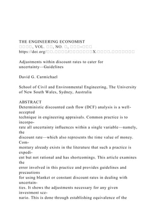
� Time into the future at which the cash flow occurs. Times
range from 1 to 10 years.
� The base interest rate, to which an additive adjustment is
made to give a discount rate.
Base interest rates range from 0.05 (5% per annum) to 0.15
(15% per annum).
� The level of risk aversion of the investor. Figure 1 shows the
utility functions used in
the analysis, ranging from risk neutral to risk averse.
(Comments only are given on risk
seeking attitudes.) These are typical utility functions,
representative of different levels of
risk aversion. The risk aversion coefficients, RA, given in
Figure 1 are those evaluated at
E[PW]. The risk aversion coefficient for a quadratic utility
function varies with the value
of PW used in its evaluation.
Demonstration of adjustments needed
Using the above analysis, Figures 2 to 7 illustrate the type of
adjustment that needs to be made
to blanket or constant discount rates where uncertainty is
present. By implication, they also
show the errors involved in assuming constant discount rates in
the presence of uncertainty.
All rate adjustments shown are additive to the base rate.
Figures 2 to 7 are examples of a much larger numerical
experimentation but represent typi-
cal results. The range of values used in the experimentation
covers typical commercial values.
Single cash flow
Figures 2 to 4 show typical results for a single cash flow

occurring at a future time. RA is the
level of risk aversion defined in Equation (3). COV is the
coefficient of variation. Base rate is
the constant discount rate to which an adjustment is applied.
Although not presented here, adjustments for the risk-seeking
case are opposite in sign to
those for the risk averse case.
Uniform cash flows
Figures 5 to 7 show typical results for a uniform series of cash
flows starting in year 1 and
proceeding variously up to year 1, 4, 7, and 10. The coefficient
of variation, COV, refers to

the cash flow at each year. Figures 5 to 7 are given for cash
flows in each year being perfectly
correlated; lesser correlation (including independence) leads to
lower adjustments.
General collection of cash flows
For a general collection of cash flows and correlation
assumptions, the analysis does not
change; however, it can be harder to isolate the influence of a
mixture of analysis inputs.
Fi
Summary
In summary, the numerical experimentation shows that
deterministic DCF analysis using
blanket discount rates does not accurately incorporate an
investment’s uncertainty. This
affects any conclusions on investment viability. The resultant
present worth calculated will
be wrongly valued.
The numerical study results can be summarized as follows:
� Risk-neutral attitudes lead to no adjustment of the base rate.
Risk-averse attitudes require
rate adjustment according to the following points.
� With increasing base interest rate, the additive adjustment

decreases slightly but is almost
constant. (As a proportion of the base rate, it decreases.)
� With increasing time, i, into the future at which the cash flow
occurs, the adjustment
decreases (with the rate of adjustment decreasing with time). No
adjustment is necessary
at long times into the future.
� With increasing uncertainty in the cash flow (as measured by
the cash flow COV), the
adjustment increases (with the rate of adjustment increasing
with COV).
� With increasing level of risk aversion, the adjustment
increases.
Depending on where the present worth expected value lies
within the utility function, the
results will change but still the trends will remain. Accordingly,
the values given in Figures 2 to
7 are not to be taken as definitive but rather as indicating
trends. To establish specific numer-
ical values, rather than trends, each investor needs its own
utility function and analysis for
each investment case.
For identical utility functions, but applying over different
magnitudes of present worth, the
form of adjustment remains unchanged for different magnitudes,
only varying with the cash
flow coefficient of variation. However, it is anticipated that
investors’ utility functions would
change, depending on the degree of risk aversion exhibited,
with increasing magnitudes of
present worth involved.

The analysis for multiple cash flows is no different than that for
a single cash flow or uni-
form series of cash flows. Some extensions can be argued (by
comparison with a single cash
flow) using Equations (1a) and 1(b) and Figures 2 to 7 to apply
to multiple cash flows.
Comparison with the literature
Existing literature analyzing the influence of uncertainty on
discount rates tends to be directed
at market-oriented investments rather than real assets as in this
article. Hence, the treatment
and categorization of uncertainty is different. The present
article looks at an investment’s
total cash flow uncertainty, rather than components of
uncertainty. In addition, different from
existing methods is the choice of the base interest rate.
Generally, market-oriented treatments
use a risk-free rate as a base. In the present article, the user is
able to select any base rate that
is considered appropriate, including the risk-free rate, WACC,
or other. The results are not
dependent on what this base rate is, unlike market-oriented
treatments.
It is believed that the present article provides a more complete
understanding of discount
rate determination in the presence of cash flow uncertainty for
real assets compared to existing
methods. Existing methods of establishing a risk-adjusted
discount rate tend to be subjective
and inconsistent (Halliwell 2001). Users attempt to
acknowledge the uncertainty associated
with cash flows with a rate adjustment that does not accurately

reflect an investment’s uncer-
tainty. A strong argument against the current practice of using
risk-adjusted discount rates is
that the adjustment adopted is a constant over time and over
different cash flows and does not
Increases in Will lead to adjustments being
Base interest rate Slightly lower; almost constant (but
proportionally lower)
The future timing of cash flows Lower
Cash flow uncertainty Higher
Risk aversion Higher
reflect the true underlying cash flow uncertainty. This article’s
results show the deficiencies in
such an approach; here it is shown that the adjustment needs to
change with level of cash flow
uncertainty, cash flow timing, and degree of risk aversion but
only mildly with base rate. With
possibly the exception of a change in the base rate, the rate
adjustments are not constant over
these variables.
The time variability of adjustments shown in Figure 2 is in
agreement with the arguments
of Weitzman (1998) and Gollier (2002), the implied rates in
Espinoza (2014) using synthetic
insurances, and the real option results of Carmichael et al.
(2011) and Carmichael (2014,

2016a). The time influences in Figure 2 also agree in form with
Robichek and Myers (1966),
Berry and Dyson (1980), Dyson and Berry (1983), Baker and
Fox (2003), and Cheremushkin
(2009). However, these papers are silent on the influence of the
base rate and cash flow vari-
ance. On the influence of the level of risk aversion, the
qualitative comments in these papers
agree with Figures 3 and 6.
The negative adjustment comment is consistent with Berry and
Dyson (1980) and Dyson
and Berry (1983).
Guidelines
In using discount rates and a deterministic DCF analysis, Table
1 gives guidelines for adjusting
the rate to take care of uncertainty in the cash flows.
These guidelines provide a rate adjustment that more accurately
represents an investment’s
cash flow uncertainty over existing methods. In order to use the
article’s findings, it is neces-
sary that users only understand their level of risk aversion
(ranging from risk neutral through
to low, medium, and high risk aversion), not that they be able to
generate their own utility
functions. For accurate adjustments for any given situation,
users should develop their own
utility function and apply their own values substituted into
Equations (1) to (4).
Conclusions
A single blanket or constant discount rate is not able to

simultaneously represent the time
value of money and uncertainty. The article shows the
limitations and errors involved in
requiring the discount rate to do this but also provides, on a
case-by-case basis, a way of
adjusting rates such that the errors are minimized. The
requirement for adjustments demon-
strates that errors are involved in using blanket discount rates.
The article’s results show that
the adjustment varies with timing of the cash flow, cash flow
uncertainty, and level of risk
aversion but only mildly with the base rate. By not
appropriately acknowledging investment
uncertainty, any conclusions on investment viability can be
questioned.
The article showed trends relating to the influence of the
underlying analysis variables. It
showed the quantitative adjustments necessary for any given
investment scenario. Generally,
it is found that the rate adjustment should be decreased as the
cash flow timing increases,
increased as the variance of the cash flows increases, kept
almost constant as the base rate
increases, and increased as the investor’s level of risk aversion
increases.
In the absence of a full probabilistic analysis, the guidelines
presented here represent a way
forward if deterministic analysis is pursued, as is the current
custom. Users are now able to

make a more informed approach to rate adjustment, rather than
it being arbitrary. The article’s
results will be useful not only for single investments but also in
the comparison of multiple
investments involving uncertain cash flows, where the cash flow
timing and uncertainty differ
across the different investments.
The numerical results are based on assumptions regarding
utility. Each person and organi-
zation has its own utility function and this can change
depending on the type and magnitude
of an investment and the range of present worth anticipated.
There is no standardized util-
ity function that can be applied to all investments. Here, typical
utility functions for different
levels of risk aversion are used. Using the theory presented in
this article, each person or orga-
nization could incorporate its own utility function and cash
flows and derive a specific rate
adjustment. The trends demonstrated in this article are not
anticipated to change, though
particular numerical values will. Utility is not totally embraced
by everyone, but it has strong
support and appears frequently in the commerce literature.
Accordingly, it is emphasized that
the article’s results have this qualification.
Further research
More extensive numerical studies could be performed to verify
the article’s results, in partic-
ular, looking at the influence of the investor’s degree of risk
aversion as represented by utility
functions. Ultimately, an aim of further research might be to
develop a function for the rate

adjustment that incorporates all of the key investment variables.
The research only accounted
for uncertainty in cash flows and assumes no uncertainty in the
base rate uncertainty
and no uncertainty in the cash flow timing. Uncertainty in the
interest rate could be included
through the results of Carmichael and Bustamante (2014). See
also Carmichael and Handford
(2015).
With present worth being calculated from a nonlinear
expression and with the quadratic
used for utility, the combined nonlinearity prevented obtaining
any closed-form result. The
rate adjustment occurs within the denominator raised to a
power. Restricted closed-form
results may, however, be possible using an exponential utility
curve.
Notes on contributor
David G. Carmichael is a Professor of Civil Engineering and
former Head of the Department of Engi-
neering Construction and Management at the University of New
South Wales, Australia. He is a grad-
uate of the Universities of Sydney and Canterbury; a Fellow of
the Institution of Engineers, Australia; a
Member of the American Society of Civil Engineers; and a
former graded arbitrator and mediator. Pro-
fessor Carmichael publishes, teaches, and consults widely in
most aspects of project management, con-
struction management, systems engineering, and problem
solving. He is known for his leftfield thinking
on project and risk management (Project Management
Framework, A. A. Balkema, Rotterdam, 2004),
project planning (Project Planning, and Control, Taylor and

Francis, London, 2006), problem solving
(Problem Solving for Engineers, CRC Press, Taylor and Francis,
London, 2013), and infrastructure invest-
ment (Infrastructure Investment: An Engineering Perspective,
CRC Press, Taylor and Francis, London,
2014).
References
Ang, A.H.-S. and Tang, W. H. (1984) Probability concepts in
engineering planning and design. Vol. 2.
John Wiley & Sons, New York.
Ariel, R. (1998) Risk adjusted discount rates and the present
value of risky costs. The Financial Review,
33(1), 17–30.
Baker, R. and Fox, R. (2003) Capital investment appraisal: a
new risk premium model. International
Transactions in Operational Research, 10(2), 115–126.
Benjamin, J.R. and Cornell, C.A. (1970) Probability, statistics,
and decision for civil engineers. McGraw-
Hill, New York.
Berry, R.H. and Dyson, R.G. (1980) On the negative risk
premium for risk adjusted discount rates.
Journal of Business Finance and Accounting, 7(3), 427–436.
Block, S. (2005) Are there differences in capital budgeting
procedures between industries? The Engi-
neering Economist, 50(1), 55–67.

Block, S. (2011) Does the weighted average cost of capital
describe the real-world approach to the dis-
count rate? The Engineering Economist, 56(2), 170–180.
Bodie, Z. (2011) Investments. 9th ed. McGraw-Hill Irwin, New
York.
Brealey, R., Myers, S. and Allen, F. (2011) Principles of
corporate finance. 10th ed. McGraw-Hill Irwin,
New York.
Brennan, M.J. (1997) The term structure of discount rates.
Financial Management, 26(1), 81–90.
Bruner, R., Eades, K., Harris, R. and Higgins, R. (1998) Best
practices in estimating the cost of capital:
survey and synthesis. Financial Practice and Education, 1, 13–
28.
Carmichael, D.G. (2014) Infrastructure investment: an
engineering perspective. CRC Press, London.
Carmichael, D.G. (2016a) A cash flow view of real options. The
Engineering Economist. [Epub ahead of
print]. Available at
http://dx.doi.org/10.1080/0013791X.2016.1157661 (accessed
April 12, 2016).
Carmichael, D.G. (2016b) Risk—a commentary. Civil
Engineering and Environmental Systems, 33(3),
177–198.
Carmichael, D.G. and Balatbat, M.C.A. (2008) Probabilistic
DCF analysis, and capital budgeting and
investment—a survey. The Engineering Economist, 53(1), 84–
102.
Carmichael, D.G. and Bustamante, B.L. (2014) Interest rate

uncertainty and investment value—a second
order moment approach. International Journal of Engineering
Management and Economics, 4(2),
176–189.
Carmichael, D.G. and Handford, L.B. (2015) A note on
equivalent fixed-rate and variable-rate loans;
borrower’s perspective. The Engineering Economist, 60(2),
155–162.
Carmichael, D.G., Hersh, A.M. and Parasu, P. (2011) Real
options estimate using probabilistic present
worth analysis. The Engineering Economist, 56(4), 295–320.
Cheremushkin, S.V. (2009) Revisiting modern discounting of
risky cash flows. Available at
http://papers.ssrn.com/sol3/papers.cfm?abstract_id=1526683
(accessed December 10, 2015).
Damodaran, A. (2001) Investment valuation. 2nd ed. John Wiley
& Sons, New York.
Damodaran, A. (2007a) Strategic risk taking: a framework for
risk management. Pearson Prentice Hall,
New York.
Damodaran, A. (2007b) Valuation approaches and metrics: a
survey of the theory and evidence. John
Wiley & Sons, New York.
Dyson, R.G. and Berry, R.H. (1983) On the negative risk
premium for risk adjusted discount rates: a
reply. Journal of Business Finance and Accounting, 10(1), 157–
159.
Espinoza, R.D. and Morris, J.W.F. (2013) Decoupled NPV: a

simple, improved method to value infras-
tructure investments. Construction Management and Economics,
31(5), 471–496.
Espinoza, R.D. (2014) Separating project risk from the time
value of money: a step toward integration
of risk management and valuation of infrastructure investments.
International Journal of Project
Management, 32(6), 1056–1073.
Fama, E.F. (1977) Risk-adjusted discount rates and capital
budgeting under uncertainty. Journal of
Financial Economics, 5(1), 3–24.
Fama, E.F. (1996) Discounting under uncertainty. The Journal
of Business, 69(4), 415–428.
Fama, E.F. and French, K. (2004) The capital asset pricing
model. Journal of Economic Perspectives, 18(3),
25–46.
Gollier, C. (2002) Time horizon and the discount rate. Journal
of Economic Theory, 107(2), 463–473.
https://doi.org/10.1080/0013791X.2016.1157661
http://papers.ssrn.com/sol3/papers.cfm?abstract_id=1526683
Halliwell, L. (2001) A critique of risk-adjusted discounting.
Paper read at 32nd International
Actuarial Studies in Non-Life Insurance Colloquium,
Washington, DC, July 8–11. Available
at
http://www.actuaires.org/ASTIN/Colloquia/Washington/Halliwe

ll.pdf. (accessed December 10,
2015).
JPMorgan. (2008) The most important number in finance: the
quest for the market risk pre-
mium. JPMorgan, New York. Available at
https://www.jpmorgan.com/cm/BlobServer/
JPMorgan_CorporateFinanceAdvisory_MostImportantNumber.p
df?blobkey=id&blobwhere=
1320675769380&blobheader=application/pdf&blobheadername1
=Cache-Control&blobheader
value1=private&blobcol=urldata&blobtable=MungoBlobs
(accessed December 10, 2015).
KPMG. (2013) Valuation practices survey, KPMG, Sydney,
Australia. Available at https://www.kpmg.
com/AU/en/IssuesAndInsights/ArticlesPublications/valuation-
practices-survey/Documents/
valuation-practices-survey-2013-v3.pdf (accessed December 10,
2015).
Lintner, J. (1965) The valuation of risk assets and the selection
of risky investments in stock portfolios
and capital budgets. Review of Economics and Statistics, 47(1),
13–37.
Markowitz, H. (2014) Mean–variance approximations to
expected utility. European Journal of Opera-
tional Research, 234(2), 346–355.
National Oceanic and Atmospherica Administration. (2014)
Discounting and time preference. National
Oceanic and Atmospheric Administration, Washington, DC.
Available at http://www.csc.noaa.gov/
archived/coastal/economics/discounting.htm (accessed
December 10, 2105)

Robichek, A.A. and Myers, S.C. (1966) Conceptual problems in
the use of risk adjusted discount rates.
The Journal of Finance, 21(4), 727–730.
Ross, S.A., Westerfield, R.W. and Jordan, B.D. (2013)
Fundamentals of corporate finance. 10th ed.
McGraw-Hill Irwin, New York.
Sharpe, W.F. (1964) Capital asset prices: a theory of market
equilibrium under conditions of risk. Journal
of Finance, 19(3), 425–442.
Weitzman, M.L. (1998) Why the far-distant future should be
discounted at its lowest possible rate. Jour-
nal of Environmental Economics and Management, 36, 201–208.
Zinn, C.D., Lesso, W.G. and Motazed, B. (1977) A probabilistic
approach to risk analysis in capital
investment projects. The Engineering Economist, 22(4), 239–
260.
http://www.actuaires.org/ASTIN/Colloquia/Washington/Halliwe
ll.pdf
https://www.jpmorgan.com/cm/BlobServer/JPMorgan_Corporate
FinanceAdvisory_MostImportantNumber.pdf?blobkey=id&blob
where=1320675769380&blobheader=application/pdf&blobheade
rname1=Cache-
Control&blobheadervalue1=private&blobcol=urldata&blobtable
=MungoBlobs
https://www.kpmg.com/AU/en/IssuesAndInsights/ArticlesPublic
ations/valuation-practices-survey/Documents/valuation-
practices-survey-2013-v3.pdf
http://www.csc.noaa.gov/archived/coastal/economics/discountin
g.htm

Copyright of Engineering Economist is the property of Taylor &
Francis Ltd and its content
may not be copied or emailed to multiple sites or posted to a
listserv without the copyright
holder's express written permission. However, users may print,
download, or email articles for
individual use.
AbstractIntroductionBackgroundRate adjustmentOther methods
of establishing discount ratesAnalysisNumerical
studiesIntroductionDemonstration of adjustments
neededSummaryComparison with the
literatureGuidelinesConclusionsFurther researchNotes on
contributorReferences

THE ENGINEERING ECONOMIST, VOL. , NO. , –http.docx

Recommended

Recommended

More Related Content

Similar to THE ENGINEERING ECONOMIST, VOL. , NO. , –http.docx

Similar to THE ENGINEERING ECONOMIST, VOL. , NO. , –http.docx (20)

More from todd701

More from todd701 (20)

Recently uploaded

Recently uploaded (20)

THE ENGINEERING ECONOMIST, VOL. , NO. , –http.docx