Decision Tree Classification

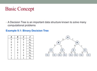
Basic Concept
• A Decision Tree is an important data structure known to solve many
computational problems
Example 9.1: Binary Decision Tree
A B C f
0 0 0 m0
0 0 1 m1
0 1 0 m2
0 1 1 m3
1 0 0 m4
1 0 1 m5
1 1 0 m6
1 1 1 m7

Basic Concept
• In Example 9.1, we have considered a decsion tree where values of
any attribute if binary only. Decision tree is also possible where
attributes are of continuous data type
Example 9.2: Decision Tree with numeric data

Some Characteristics
• Decision tree may be n-ary, n ≥ 2.
• There is a special node called root node.
• All nodes drawn with circle (ellipse) are called internal nodes.
• All nodes drawn with rectangle boxes are called terminal nodes or leaf
nodes.
• Edges of a node represent the outcome for a value of the node.
• In a path, a node with same label is never repeated.
• Decision tree is not unique, as different ordering of internal nodes can
give different decision tree.

Decision Tree and Classification Task
• Decision tree helps us to classify data.
• Internal nodes are some attribute
• Edges are the values of attributes
• External nodes are the outcome of classification
• Such a classification is, in fact, made by posing questions starting from
the root node to each terminal node.

Example 9.3 : Vertebrate Classification
What are the class label of Dragon and Shark?
Name Body
Temperature
Skin
Cover
Gives
Birth
Aquatic
Creature
Aerial
Creature
Has
Legs
Hibernates Class
Human Warm hair yes no no yes no Mammal
Python Cold scales no no no no yes Reptile
Salmon Cold scales no yes no no no Fish
Whale Warm hair yes yes no no no Mammal
Frog Cold none no semi no yes yes Amphibian
Komodo Cold scales no no no yes no Reptile
Bat Warm hair yes no yes yes yes Mammal
Pigeon Warm feathers no no yes yes no Bird
Cat Warm fur yes no no yes no Mammal
Leopard Cold scales yes yes no no no Fish
Turtle Cold scales no semi no yes no Reptile
Penguin Warm feathers no semi no yes no Bird
Porcupine Warm quills yes no no yes yes Mammal
Eel Cold scales no yes no no no Fish
Salamander Cold none no semi no yes yes Amphibian

Example 9.3 : Vertebrate Classification
• Suppose, a new species is discovered as follows.
• Decision Tree that can be inducted based on the data (in Example 9.3)
is as follows.
Name Body
Temperature
Skin
Cover
Gives
Birth
Aquatic
Creature
Aerial
Creature
Has
Legs
Hibernates Class
Gila Monster cold scale no no no yes yes
?

• Example 9.3 illustrates how we can solve a classification problem by
asking a series of question about the attributes.
• Each time we receive an answer, a follow-up question is asked until we reach
a conclusion about the class-label of the test.
• The series of questions and their answers can be organized in the form
of a decision tree
• As a hierarchical structure consisting of nodes and edges
• Once a decision tree is built, it is applied to any test to classify it.

Definition of Decision Tree
Given a database D = 𝑡1, 𝑡2, … . . , 𝑡𝑛 , where 𝑡𝑖 denotes a tuple, which is
defined by a set of attribute 𝐴 = 𝐴1, 𝐴2, … . . , 𝐴𝑚 . Also, given a set of
classes C = 𝑐1, 𝑐2, … . . , 𝑐𝑘 .
A decision tree T is a tree associated with D that has the following
properties:
• Each internal node is labeled with an attribute Ai
• Each edges is labeled with predicate that can be applied to the attribute
associated with the parent node of it
• Each leaf node is labeled with class cj
Definition 9.1: Decision Tree

Building Decision Tree
• In principle, there are exponentially many decision tree that can be
constructed from a given database (also called training data).
• Some of the tree may not be optimum
• Some of them may give inaccurate result
• Two approaches are known
• Greedy strategy
• A top-down recursive divide-and-conquer
• Modification of greedy strategy
• ID3
• C4.5
• CART, etc.

Built Decision TreeAlgorithm
Algorithm: Generate decision tree. Generate a decision tree from the training tuples of data partition, D. Input:
Data partition, D, which is a set of training tuples and their associated class labels;
attribute list, the set of candidate attributes;
Attribute selection method, a procedure to determine the splitting criterion that “best” partitions the data tuples
into individual classes. This criterion consists of a splitting attribute and, possibly, either a split-point or splitting
subset.
Output: A decision tree.
Method:
(1) create a node N;
(2) if tuples in D are all of the same class, C, then
(3) return N as a leaf node labeled with the class C;
(4) if attribute list is empty then
(5) return N as a leaf node labeled with the majority class in D; // majority voting
(6) apply Attribute selection method(D, attribute list) to find the “best” splitting criterion;
(7) label node N with splitting criterion;
(8) if splitting attribute is discrete-valued and multiway splits allowed then // not restricted to binary trees
(9) attribute list ← attribute list − splitting attribute; // remove splitting attribute
(10) for each outcome j of splitting criterion // partition the tuples and grow subtrees for each partition
(11) let Dj be the set of data tuples in D satisfying outcome j; // a partition
(12) if Dj is empty then
(13) attach a leaf labeled with the majority class in D to node N;
(14) else attach the node returned by Generate decision tree(Dj , attribute list) to node N; endfor

Node Splitting in BuildDTAlgorithm
• BuildDT algorithm must provides a method for expressing an attribute test
condition and corresponding outcome for different attribute type
• Case: Binary attribute
• This is the simplest case of node splitting
• The test condition for a binary attribute generates only two outcomes

• Case: Nominal attribute
• Since a nominal attribute can have many values, its test condition can be expressed in
two ways:
• A multi-way split
• A binary split
• Muti-way split: Outcome depends on the number of distinct values for the
corresponding attribute
• Binary splitting by grouping attribute values

• Case: Ordinal attribute
• It also can be expressed in two ways:
• A multi-way split
• A binary split
• Muti-way split: It is same as in the case of nominal attribute
• Binary splitting attribute values should be grouped maintaining the order property of
the attribute values

• Case: Numerical attribute
• For numeric attribute (with discrete or continuous values), a test condition can be
expressed as a comparison set
• Binary outcome: A > v or A ≤ v
• In this case, decision tree induction must consider all possible split positions
• Range query : vi ≤ A < vi+1 for i = 1, 2, …, q (if q number of ranges are chosen)
• Here, q should be decided a priori
• For a numeric attribute, decision tree induction is a combinatorial optimization
problem

Illustration : BuildDTAlgorithm
Example 9.4: Illustration of BuildDT Algorithm
• Consider a training data set as shown.
Person Gender Height Class
1 F 1.6 S
2 M 2.0 M
3 F 1.9 M
4 F 1.88 M
5 F 1.7 S
6 M 1.85 M
7 F 1.6 S
8 M 1.7 S
9 M 2.2 T
10 M 2.1 T
11 F 1.8 M
12 M 1.95 M
13 F 1.9 M
14 F 1.8 M
15 F 1.75 S
Attributes:
Gender = {Male(M), Female (F)} // Binary attribute
Height = {1.5, …, 2.5} // Continuous
attribute
Class = {Short (S), Medium (M), Tall (T)}
Given a person, we are to test in which class s/he
belongs

• To built a decision tree, we can select an attribute in two different orderings:
<Gender, Height> or <Height, Gender>
• Further, for each ordering, we can choose different ways of splitting
• Different instances are shown in the following.
• Approach 1 : <Gender, Height>

• Approach 2 : <Height, Gender>

Example 9.5: Illustration of BuildDT Algorithm
• Consider an anonymous database as shown.
A1 A2 A3 A4 Class
a11 a21 a31 a41 C1
a12 a21 a31 a42 C1
a11 a21 a31 a41 C1
a11 a22 a32 a41 C2
a11 a22 a32 a41 C2
a12 a22 a31 a41 C1
a11 a22 a32 a41 C2
a11 a22 a31 a42 C1
a11 a21 a32 a42 C2
a11 a22 a32 a41 C2
a12 a22 a31 a41 C1
a12 a22 a31 a42 C1
• Is there any “clue” that enables to
select the “best” attribute first?
• Suppose, following are two
attempts:
• A1A2A3A4 [naïve]
• A3A2A4A1 [Random]
• Draw the decision trees in the above-
mentioned two cases.
• Are the trees different to classify any test
data?
• If any other sample data is added into the
database, is that likely to alter the decision
tree already obtained?

Concept of Entropy
If a point represents a gas molecule,
then which system has the more
entropy?
How to measure? ∆𝑆 =
∆𝑄
𝑇
?
More organized or Less organized or
ordered (less probable) disordered (more probable)
More ordered Less ordered
less entropy higher entropy

Concept of Entropy
Universe!
What was its entropy value at its starting point?

An Open Challenge!
Two sheets showing the tabulation of marks obtained in a course
are shown.
Which tabulation of marks shows the “good” performance of the
class?
How you can measure the same?
Roll No. Assignment Project Mid-Sem End-Sem
12BT3FP06 89 99 56 91
10IM30013 95 98 55 93
12CE31005 98 96 58 97
12EC35015 93 95 54 99
12GG2005 90 91 53 98
12MI33006 91 93 57 97
13AG36001 96 94 58 95
13EE10009 92 96 56 96
13MA20012 88 98 59 96
14CS30017 94 90 60 94
14ME10067 90 92 58 95
14MT10038 99 89 55 93
Roll No. Assignment Project Mid-Sem End-Sem
12BT3FP06 19 59 16 71
10IM30013 37 38 25 83
12CE31005 38 16 48 97
12EC35015 23 95 54 19
12GG2005 40 71 43 28
12MI33006 61 93 47 97
13AG36001 26 64 48 75
13EE10009 92 46 56 56
13MA20012 88 58 59 66
14CS30017 74 20 60 44
14ME10067 50 42 38 35
14MT10038 29 69 25 33

Entropy and its Meaning
• Entropy is an important concept used in Physics in the context of heat
and thereby uncertainty of the states of a matter.
• At a later stage, with the growth of Information Technology, entropy
becomes an important concept in Information Theory.
• To deal with the classification job, entropy is an important concept,
which is considered as
• an information-theoretic measure of the “uncertainty” contained in a
training data
• due to the presence of more than one classes.

Entropy in Information Theory
• The entropy concept in information theory first time coined by Claude
Shannon (1850).
• The first time it was used to measure the “information content” in messages.
•
• According to his concept of entropy, presently entropy is widely being used as
a way of representing messages for efficient transmission by
Telecommunication Systems.

Measure of Information Content
• People, in general, are information hungry!
• Everybody wants to acquire information (from newspaper, library, nature,
fellows, etc.)
• Think how a crime detector do it to know about the crime from crime spot and
criminal(s).
• Kids annoyed their parents asking questions.
• In fact, fundamental thing is that we gather information asking questions (and
decision tree induction is no exception).
•
• We may note that information gathering may be with certainty or uncertainty.

Measure of Information Content
Example 9.6
a) Guessing a birthday of your classmate
It is with uncertainty ~
1
365
Whereas guessing the day of his/her birthday is
1
7
.
This uncertainty, we may say varies between 0 to 1, both inclusive.
b) As another example, a question related to event with eventuality (or
impossibility) will be answered with 0 or 1 uncertainty.
• Does sun rises in the East? (answer is with 0 uncertainty)
• Will mother give birth to male baby? (answer is with ½ uncertainty)
• Is there a planet like earth in the galaxy? (answer is with an extreme uncertainty)

Definition of Entropy
Suppose there are m distinct objects, which we want to identify by asking a
series of Yes/No questions. Further, we assume that m is an exact power of 2, say
𝑚 = 2𝑛, where 𝑛 ≥ 1.
The entropy of a set of m distinct values is the minimum number of yes/no
questions needed to determine an unknown values from these m possibilities.
Definition 9.2: Entropy

Entropy Calculation
• How can we calculate the minimum number of questions, that is,
entropy?
• There are two approaches:
• Brute –force approach
• Clever approach.
Example 9.7: City quiz
Suppose, Thee is a quiz relating to guess a city out of 8 cities, which are as follows:
Bangalore, Bhopal, Bhubaneshwar, Delhi, Hyderabad, Kolkata, Madras, Mumbai
The question is, “Which city is called city of joy”?

Approach 1: Brute-force search
• Brute force approach
• We can ask “Is it city X?”,
• if yes stop, else ask next …
In this approach, we can ask such questions randomly choosing one city at a time. As a
matter of randomness, let us ask the questions, not necessarily in the order, as they are in
the list.
Q.1: Is the city Bangalore? No
Q.2: Is the city Bhubaneswar? No
Q.3: Is the city Bhopal? No
Q.4: Is the city Delhi? No
Q.5: Is the city Hyderabad? No
Q.6: Is the city Madras? No
Q.7: Is the city Mumbai? No
No need to ask further question! Answer is already out by the Q.7. If asked randomly,
each of these possibilities is equally likely with probability
1
8
. Hence on the average, we
need
(1+2+3+4+5+6+7+7)
8
= 4.375 questions.

Approach 2: Clever approach
• Clever approach (binary search)
• In this approach, we divide the list into two halves, pose a question for a half
• Repeat the same recursively until we get yes answer for the unknown.
Q.1: Is it Bangalore, Bhopal, Bhubaneswar or Delhi? No
Q.2: Is it Madras or Mumbai? No
Q.3: Is it Hyderabad? No
So after fixing 3 questions, we are able to crack the answer.
Note:
Approach 2 is considered to be the best strategy because it will invariably find the answer and
will do so with a minimum number of questions on the average than any other strategy.
Approach 1 occasionally do better (when you are lucky enough!)
• It is no coincidence that 8 = 23
, and the minimum number of yes/no questions needed is 3.
• If m = 16, then 16 = 24
, and we can argue that we need 4 questions to solve the problem. If
m = 32, then 5 questions, m = 256, then 8 questions and so on.

The minimum number of yes/no questions needed to identify an unknown
object from 𝑚 = 2𝑛 equally likely possible object is n.
If m is not a power of 2, then the entropy of a set of m distinct objects that
are equally likely is log2 𝑚
Lemma 9.1: Entropy calculation
Entropy Calculation

Entropy in Messages
• We know that the most conventional way to code information is using binary bits, that
is, using 0s and 1s.
• The answer to a question that can only be answered yes/no (with equal probability) can
be considered as containing one unit of information, that is, one bit.
• In other words, the unit of information can also be looked at as the amount of
information that can be coded using only 0s and 1s.

Entropy in Messages
Example 9.7: Information coding
• If we have two possible objects say male and female, then we use the coding
0 = female
1 = male
• We can encode four possible objects say East, West, North, South using two bits, for example
00 : North
01 : East
10 : West
11 : South
• We can encode eight values say eight different colours, we need to use three bits, such as
000 : Violet
001 : Indigo
010 : Blue
011 : Green
100 : Yellow
101 : Orange
110 : Red
111 : White
Thus, in general, to code m values, each in a distinct manner, we need n bits such that 𝑚 = 2𝑛
.
𝑚 = 2(= 2𝑛
, 𝑛 = 1)
𝑚 = 4(= 2𝑛
, 𝑛 = 2)
𝑚 = 8(= 2𝑛
, 𝑛 = 3)

Entropy in Messages
• In this point, we can note that to identify an object, if it is encoded with bits, then we
have to ask questions in an alternative way. For example
• Is the first bit 0?
• Is the second bit 0?
• Is the third bit 0? and so on
• Thus, we need n questions, if m objects are there such that 𝑚 = 2𝑛.
• The above leads to (an alternative) and equivalent definition of entropy
The entropy of a set of m distinct values is the number of bits needed to encode all
the values in the most efficient way.
Definition 9.3: Entropy

Messages when (𝑚 ≠ 2𝑛
)
• In the previous discussion, we have assumed that m, the number of distinct objects is exactly
a power of 2, that is 𝑚 = 2𝑛
for some 𝑛 ≥ 1 and all m objects are equally likely.
• This is mere an assumption to make the discussion simplistic.
• In the following we try to redefine the entropy calculation in more general case, that is, when
m ≠ 2𝑛
and not necessarily m objects are equally probable. Let us consider a different
instance of yes/no question game, which is as follows.
Example 9.8: Name game
• There are seven days: Sun, Mon, Tue, Wed, Thu, Fri, Sat.
•
• We are to identify a sequence of 𝑘 ≥ 1 such values (each one chosen independently of the others, that
is, repetitions are allowed). Note that if k = 1, it is the type of game, we have already dealt with.
• We denote the minimum number of 𝑦𝑒𝑠/𝑛𝑜 questions needed to identify a sequence of 𝑘 unknown
values drawn independently from 𝑚 possibilities as 𝐸𝑘
𝑚
, the entropy in this case.
• In other words, 𝐸𝑘
𝑚
is the number of questions required to discriminate amongst 𝑚𝑘
distinct
possibilities.

Messages when (𝑚 ≠ 2𝑛
)
• Here, 𝑚 = 7 (as stated in the game of sequence of days) and k = 6 (say).
• An arbitrary sequence may be {Tue, Thu, Tue, Mon, Sun, Tue}, etc. There are 76
= 117649
possible sequences of six days.
• From our previous understanding, we can say that the minimum number of 𝑦𝑒𝑠/𝑛𝑜 questions that
is required to identify such a sequence is log2 11769 = 16.8443.
• Since, this is a non integer number, and the number of question should be an integer, we can say
17 questions are required. Thus,
𝐸6
7
= log2 76
• In general,
𝐸𝑘
𝑚
= log2 𝑚𝑘
• Alternatively, the above can be written as,
log2 𝑚𝑘
≤ 𝐸𝑘
𝑚
≤ log2 𝑚𝑘
+ 1
• Or
log2 𝑚 ≤
𝐸𝑘
𝑚
𝑘
≤ log2 𝑚 +
1
𝑘

Entropy of Messages when (𝑚 ≠ 2𝑛
)
Note that here
𝐸𝑘
𝑚
𝑘
is the average number of questions needed to determine each of the
values in a sequence of k values. By choosing a large enough value of k, that is, a long
enough sequence, the value of
1
𝑘
can be made as small as we wish. Thus, the average
number of questions required to determine each value can be made arbitrarily close to
log2 𝑚. This is evident from our earlier workout, for example, tabulated below, for m = 7.
𝐸𝑘
𝑚
= log2 𝑚𝑘
k 𝑚𝑘
log2 𝑚𝑘 No. Q 𝑵𝒐. 𝑸
𝑘
6 117649 16.84413 17 2.8333
21 58.95445 59 2.8095
1000 2807.3549 2808 2.8080
….. ….. ….. ….. …..
No. Q = Number of questions
Note that log2 7 ≈ 2.8074 and
𝑵𝒐.𝑸
𝑘
≈ log2 7. Further,
𝑵𝒐.𝑸
𝑘
=
𝐸𝑘
7
𝑘
i.e.
𝐸𝑘
7
𝑘
= log2 7 (is
independent of k and is a constant!)

Entropy of Messages when (𝑚 ≠ 2𝑛
)
The entropy of a set of m distinct objects is log2 𝑚 even when m is not exactly a
power of 2.
• We have arrived at a conclusion that E = log2 𝑚 for any value of m, irrespective of
weather it is a power of 2 or not.
Note: E is not necessarily be an integer always.
• Next, we are to have our observation, if all m objects are not equally probable.
• Suppose, 𝑝𝑖 denotes the frequency with which the 𝑖𝑡ℎ
of the m objects occurs,
where 0 ≤ 𝑝𝑖 ≤ 1 for all 𝑝𝑖 such that
𝑖=1
𝑚
𝑝𝑖 = 1
Lemma 9.4: Entropy Calculation

Discriminating amongst m values (𝑚 ≠ 2𝑛
)
Example 9.8: Discriminating among objects
• Suppose four objects 𝐴, 𝐵, 𝐶 𝑎𝑛𝑑 𝐷 which occur with frequencies
1
2
,
1
4
,
1
8
and
1
8
,
respectively.
• Thus, in this example, 𝑚 = 4 and 𝑝1 =
1
2
, 𝑝2 =
1
4
, 𝑝3 =
1
8
and 𝑝4 =
1
8
.
• Using standard 2-bit encoding, we can represent them as 𝐴 = 00, 𝐵 = 01, 𝐶 = 10,
𝐷 = 11.
• Also, we can follow variable length coding (also called Huffman coding) as an
improved way of representing them.
• The Huffman coding of 𝐴, 𝐵, 𝐶 𝑎𝑛𝑑 𝐷 with their frequencies
1
2
,
1
4
,
1
8
and
1
8
are shown
below.
A = 1
B = 01
C = 001
D = 000

)
• With the above representation say, if A is to be identified, then we need to
examine only one question, for B it is 2 and for C and D both, it is 3.
• Thus, on the average, we need
1
2
× 1 +
1
4
× 2 +
1
8
× 3 +
1
8
× 3 = 1.75 𝑏𝑖𝑡𝑠
• This is the number of yes/no questions to identify any one of the four
objects, whose frequency of occurrences are not uniform.
• This is simply in contrast to 2-bit encoding, where we need 2-bits (questions)
on the average.

)
• It may be interesting to note that even with variable length encoding, there are
several ways of encoding. Few of them are given below.
• The calculation of entropy in the observed cases can be obtained as:
• Anyway, key to finding the most efficient way of encoding is to assign a
smallest number of bits to the object with highest frequency and so on.
• The above observation is also significant in the sense that it provides a
systematic way of finding a sequence of well-chosen question in order
to identify an object at a faster rate.
1) 𝐴 = 0 2) 𝐴 = 01 3) 𝐴 = 101
𝐵 = 11 𝐵 = 1 𝐵 = 001
𝐶 = 100 𝐶 = 001 𝐶 = 10011
𝐷 = 101 𝐷 = 000 𝐷 = 100001
1) 1.75 2) 2 3) 3.875

Information Content
If an object occurs with frequency p, then the most efficient way to represent it
with log2(1
𝑝) bits.
Lemma 9.3: Information content
Example 9.9: Information content
• A which occurs with frequency
1
2
is represented by 1-bit, B which occurs with
frequency
1
4
represented by 2-bits and both C and D which occurs with frequency
1
8
are represented by 3 bits each.
Based on the previous discussion we can easily prove the following lemma.

Entropy Calculation
If pi denotes the frequencies of occurrences of m distinct objects, then the entropy
E is
𝐸 =
𝑖=1
𝑚
𝑝𝑖 log(1
𝑝𝑖
) 𝑎𝑛𝑑
𝑖=1
𝑚
𝑝𝑖 = 1
Theorem 9.4: Entropy calculation
We can generalize the above understanding as follows.
• If there are m objects with frequencies 𝑝1, 𝑝2……., 𝑝𝑚, then the average number of
bits (i.e. questions) that need to be examined a value, that is, entropy is the frequency
of occurrence of the 𝑖𝑡ℎ
value multiplied by the number of bits that need to be
determined, summed up values of 𝑖 from 1 to m.
Note:
• If all are equally likely, then 𝑝𝑖 =
1
𝑚
and 𝐸 = log2 𝑚; it is the special case.

Entropy of a Training Set
• If there are k classes 𝑐1, 𝑐2……., 𝑐𝑘 and 𝑝𝑖 for 𝑖 = 1 𝑡𝑜 𝑘 denotes the number of
occurrences of classes 𝑐𝑖 divided by the total number of instances (i.e., the frequency
of occurrence of 𝑐𝑖) in the training set, then entropy of the training set is denoted by
𝐸 = −
𝑖=1
𝑚
𝑝𝑖 log2 𝑝𝑖
Here, E is measured in “bits” of information.
Note:
• The above formula should be summed over the non-empty classes only, that is, classes
for which 𝑝𝑖 ≠ 0
• E is always a positive quantity
• E takes it’s minimum value (zero) if and only if all the instances have the same class
(i.e., the training set with only one non-empty class, for which the probability 1).
• Entropy takes its maximum value when the instances are equally distributed among k
possible classes. In this case, the maximum value of E is 𝑙𝑜𝑔2 𝑘.

Entropy of a Training Set
Example 9.10: OPTH dataset
Consider the OTPH data shown in the following table with total 24 instances in it.
Age Eye sight Astigmatic Use Type Class
1
1
1
1
1
1
1
1
1
1
2
2
1
1
2
2
1
1
1
2
1
2
1
2
3
2
3
1
3
2
1
1
2
2
2
2
2
2
1
1
1
1
2
2
1
1
2
2
1
2
1
2
1
2
3
1
3
2
3
1
2
2
2
2
3
3
2
2
2
2
1
1
1
1
2
2
1
1
1
2
1
2
1
2
3
2
3
3
3
3
3
3
3
3
3
3
1
1
2
2
2
2
2
2
1
1
2
2
1
2
1
2
1
2
3
1
3
2
3
3
A coded
forms for all
values of
attributes
are used to
avoid the
cluttering in
the table.

Entropy of a training set
Specification of the attributes are as follows.
Age Eye Sight Astigmatic Use Type
1: Young 1: Myopia 1: No 1: Frequent
2: Middle-aged 2: Hypermetropia 2: Yes 2: Less
3: Old
Class: 1: Contact Lens 2:Normal glass 3: Nothing
In the OPTH database, there are 3 classes and 4 instances with class 1, 5 instances
with class 2 and 15 instances with class 3. Hence, entropy E of the database is:
𝐸 = −
4
24
log2
4
24
−
5
24
log2
5
24
−
15
24
log2
15
24
= 1.3261

Note:
• The entropy of a training set implies the number of yes/no questions, on the average,
needed to determine an unknown test to be classified.
• It is very crucial to decide the series of questions about the value of a set of attribute,
which collectively determine the classification. Sometimes it may take one question,
sometimes many more.
• Decision tree induction helps us to ask such a series of questions. In other words, we
can utilize entropy concept to build a better decision tree.
How entropy can be used to build a decision tree is our next topic of discussion.

Decision Tree Induction Techniques
• Decision tree induction is a top-down, recursive and divide-and-conquer
approach.
• The procedure is to choose an attribute and split it into from a larger training set
into smaller training sets.
• Different algorithms have been proposed to take a good control over
1. Choosing the best attribute to be splitted, and
2. Splitting criteria
• Several algorithms have been proposed for the above tasks. In this lecture, we
shall limit our discussions into three important of them
• ID3
• C 4.5
• CART

ID3: Decision Tree InductionAlgorithms
• Quinlan [1986] introduced the ID3, a popular short form of Iterative
Dichotomizer 3 for decision trees from a set of training data.
• In ID3, each node corresponds to a splitting attribute and each arc is a possible
value of that attribute.
• At each node, the splitting attribute is selected to be the most informative
among the attributes not yet considered in the path starting from the root.

Algorithm ID3
• In ID3, entropy is used to measure how informative a node is.
• It is observed that splitting on any attribute has the property that average entropy of
the resulting training subsets will be less than or equal to that of the previous
training set.
• ID3 algorithm defines a measurement of a splitting called Information Gain
to determine the goodness of a split.
• The attribute with the largest value of information gain is chosen as the splitting
attribute and
• it partitions into a number of smaller training sets based on the distinct values of
attribute under split.

Defining Information Gain
• We consider the following symbols and terminologies to define
information gain, which is denoted as α.
• D ≡ denotes the training set at any instant
• |D| ≡ denotes the size of the training set D
• E(D) ≡ denotes the entropy of the training set D
• The entropy of the training set D
E(D) = - 𝑖=1
𝑘
𝑝𝑖 𝑙𝑜𝑔2(𝑝𝑖
• where the training set D has 𝑐1, 𝑐2, … , 𝑐𝑘, the k number of distinct classes and
• 𝑝𝑖, 0< 𝑝𝑖≤ 1 is the probability that an arbitrary tuple in D belongs to class 𝑐𝑖 (i = 1,
2, … , k).

• pi can be calculated as
𝑝𝑖 =
|𝐶𝑖,𝐷|
|𝐷|
• where 𝐶𝑖,𝐷 is the set of tuples of class 𝑐𝑖 in D.
• Suppose, we want to partition D on some attribute A having m distinct values
{𝑎1, 𝑎2, … , 𝑎𝑚}.
• Attribute 𝐴 can be considered to split D into m partitions {𝐷1, 𝐷2, … , 𝐷𝑚},
where 𝐷𝑗 (j = 1,2, … ,m) contains those tuples in D that have outcome 𝑎𝑗 of A.

The weighted entropy denoted as 𝐸𝐴(𝐷) for all partitions of D with respect to A is
given by:
𝐸𝐴(𝐷) = 𝑗=1
𝑚 |𝐷𝑗|
|𝐷|
E(𝐷𝑗)
Here, the term
|𝐷𝑗|
|𝐷|
denotes the weight of the j-th training set.
More meaningfully, 𝐸𝐴(𝐷) is the expected information required to classify a tuple
from D based on the splitting of A.
Definition 9.4: Weighted Entropy

• Our objective is to take A on splitting to produce an exact classification (also
called pure), that is, all tuples belong to one class.
• However, it is quite likely that the partitions is impure, that is, they contain
tuples from two or more classes.
• In that sense, 𝐸𝐴(𝐷) is a measure of impurities (or purity). A lesser value of
𝐸𝐴(𝐷) implying more power the partitions are.
Information gain, 𝛼 𝐴, 𝐷 of the training set D splitting on the attribute A is given
by
𝛼 𝐴, 𝐷 = E(D) - 𝐸𝐴(𝐷)
In other words, 𝛼 𝐴, 𝐷 gives us an estimation how much would be gained by
splitting on A. The attribute A with the highest value of 𝛼 should be chosen as the
splitting attribute for D.
Definition 9.5: Information Gain

Information Gain Calculation
Example 9.11 : Information gain on splitting OPTH
• Let us refer to the OPTH database discussed in Slide #48.
• Splitting on Age at the root level, it would give three subsets 𝐷1, 𝐷2 and 𝐷3 as
shown in the tables in the following three slides.
• The entropy 𝐸(𝐷1), 𝐸(𝐷2) and 𝐸(𝐷3) of training sets 𝐷1, 𝐷2 and 𝐷3 and
corresponding weighted entropy 𝐸𝐴𝑔𝑒(𝐷1), 𝐸𝐴𝑔𝑒(𝐷2) and 𝐸𝐴𝑔𝑒(𝐷3) are also
shown alongside.
• The Information gain 𝛼 (𝐴𝑔𝑒, 𝑂𝑃𝑇𝐻) is then can be calculated as 0.0394.
• Recall that entropy of OPTH data set, we have calculated as E(OPTH) =
1.3261
(see Slide #49)

Information Gain Calculation
Example 9.11 : Information gain on splitting OPTH
Training set: 𝐷1(Age = 1)
Age Eye-sight Astigmatism Use type Class
1 1 1 1 3
1 1 1 2 2
1 1 2 1 3
1 1 2 2 1
1 2 1 1 3
1 2 1 2 2
1 2 2 1 3
1 2 2 2 1
𝐸(𝐷1) = −
2
8
𝑙𝑜𝑔2(
2
8
) −
2
8
𝑙𝑜𝑔2(
2
8
)
−
4
8
𝑙𝑜𝑔2(
4
8
) = 1.5
𝐸𝐴𝑔𝑒(𝐷1) =
8
24
× 1.5 = 0.5000

Calculating Information Gain
2 1 1 1 3
2 1 1 2 2
2 1 2 1 3
2 1 2 2 1
2 2 1 1 3
2 2 1 2 2
2 2 2 1 3
2 2 2 2 3
𝐸(𝐷2) = −
1
8
𝑙𝑜𝑔2(
1
8
) −
2
8
𝑙𝑜𝑔2(
2
8
) −
5
8
𝑙𝑜𝑔2(
5
8
)
= 1.2988
8
24
× 1.2988 = 0.4329

Calculating Information Gain
3 1 1 1 3
3 1 1 2 3
3 1 2 1 3
3 1 2 2 1
3 2 1 1 3
3 2 1 2 2
3 2 2 1 3
3 2 2 2 3
𝛼 (𝐴𝑔𝑒, 𝐷) = 1.3261 – (0.5000 + 0.4329 + 0.3504) = 0.0394
𝐸(𝐷3) = −
1
8
𝑙𝑜𝑔2(
1
8
) −
1
8
𝑙𝑜𝑔2(
1
8
)
−
6
8
𝑙𝑜𝑔2(
6
8
) = 1.0613
8
24
× 1.0613 = 0.3504

Information Gains for DifferentAttributes
• In the same way, we can calculate the information gains, when splitting the
OPTH database on Eye-sight, Astigmatic and Use Type. The results are
summarized below.
• Splitting attribute: Age
𝛼 𝐴𝑔𝑒, 𝑂𝑃𝑇𝐻 = 0.0394
• Splitting attribute: Eye-sight
𝛼 𝐸𝑦𝑒 − 𝑠𝑖𝑔ℎ𝑡, 𝑂𝑃𝑇𝐻 = 0.0395
• Splitting attribute: Astigmatic
𝛼 Astigmatic , 𝑂𝑃𝑇𝐻 = 0.3770
• Splitting attribute: Use Type
𝛼 Use Type , 𝑂𝑃𝑇𝐻 = 0.5488

Decision Tree Induction : ID3 Way
• The ID3 strategy of attribute selection is to choose to split on the attribute that
gives the greatest reduction in the weighted average entropy
• The one that maximizes the value of information gain
• In the example with OPTH database, the larger values of information gain is
𝛼 Use Type , 𝑂𝑃𝑇𝐻 = 0.5488
• Hence, the attribute should be chosen for splitting is “Use Type”.
• The process of splitting on nodes is repeated for each branch of the evolving
decision tree, and the final tree, which would look like is shown in the following
slide and calculation is left for practice.

Decision Tree Induction : ID3 Way
Age Eye-sight Astigmatic
𝑂𝑃𝑇𝐻
Use Type
Age Eye Ast Use Class
1 1 1 1 3
1 1 2 1 3
1 2 1 1 3
1 2 2 1 3
2 1 1 1 3
2 2 1 1 3
2 2 2 1 3
3 1 1 1 3
3 1 2 1 3
3 2 1 1 3
3 2 2 1 3
Age Eye Ast Use Class
1 1 1 2 2
1 1 2 2 1
1 2 1 2 2
1 2 2 2 1
2 1 1 2 2
2 1 2 2 1
2 2 1 2 2
3 1 1 2 3
3 1 2 2 3
3 2 1 2 2
3 2 2 2 3
× × ×

𝐹𝑟𝑒𝑞𝑢𝑒𝑛𝑡(1) 𝐿𝑒𝑠𝑠(2)
𝐷1 𝐷2
𝛼 = 0.0394 𝛼 = 0.395 𝛼 = 0.0394
𝐸(𝐷1) =? 𝐸(𝐷2) =?
𝑬 𝑶𝑷𝑻𝑯 = 𝟏. 𝟑𝟐𝟔𝟏
Age Eye-
sight
Astigmatic Age Eye-
sight
Astigmatic
? ? ? ? ? ?
𝛼 =? 𝛼 =? 𝛼 =? 𝛼 =? 𝛼 =? 𝛼 =?
𝛼 = 0.3770

Frequency Table : Calculating α
• Calculation of entropy for each table and hence information gain for a
particular split appears tedious (at least manually)!
• As an alternative, we discuss a short-cut method of doing the same using a
special data structure called Frequency Table.
• Frequency Table: Suppose, 𝑋 = {𝑥1, 𝑥2 , … , 𝑥𝑛} denotes an attribute with
𝑛 − 𝑑𝑖𝑓𝑓𝑒𝑟𝑒𝑛𝑡 attribute values in it. For a given database 𝐷, there are a set
of 𝑘 𝑐𝑙𝑎𝑠𝑠𝑒𝑠 say 𝐶 = {𝑐1, 𝑐2, … 𝑐𝑘}. Given this, a frequency table will look
like as follows.

Frequency Table : Calculating α
𝑥1 𝑥2 𝑥𝑖 𝑥𝑛
𝑐1
𝑐2
𝑐𝑗 𝑓𝑖𝑗
𝑐𝑘
Class
𝑋
• Number of rows = Number
of classes
• Number of columns =
Number of attribute values
• 𝑓𝑖𝑗 = Frequency of 𝑥𝑖 for
class 𝑐𝑗
Assume that 𝐷 = 𝑁, the number of total instances of 𝐷.

Calculation of α using Frequency Table
Example 9.12 : OTPH Dataset
With reference to OPTH dataset, and for the attribute Age, the frequency table would
look like
Column Sums
Age=1 Age=2 Age=3 Row Sum
Class 1 2 1 1 4
Class 2 2 2 1 5
Class 3 4 5 6 15
Column
Sum
8 8 8 24
N=24

Calculation of α using Frequency Table
• The weighted average entropy 𝐸𝑋(𝐷) then can be calculated from the
frequency table following the
• Calculate 𝑉 = 𝑓𝑖𝑗 log2 𝑓𝑖𝑗 for all 𝑖 = 1,2, … , 𝑘
(Entry Sum) 𝑗 = 1, 2, … , 𝑛 and 𝑣𝑖𝑗 ≠ 0
• Calculate 𝑆 = 𝑠𝑖 log2 𝑠𝑖 for all 𝑖 = 1, 2, … , 𝑛
(Column Sum) in the row of column sum
• Calculate 𝐸𝑋 𝐷 = (−𝑉 + 𝑆)/𝑁
Example 9.13: OTPH Dataset
For the frequency table in Example 9.12, we have
𝑉
= 2 log 2 + 1 log 1 + 1 log 1 + 2 log 2 + 2 log 2 + 1 log 1 + 4 log 4 + 5 log 5
+ 6 log 6
𝑆 = 8 log 8 + 8 log 8 + 8 log 8
𝑬𝑨𝒈𝒆 𝑶𝑷𝑻𝑯 = 𝟏. 𝟐𝟖𝟔𝟕

Proof of Equivalence
• In the following, we prove the equivalence of the short-cut of entropy
calculation using Frequency Table.
• Splitting on an attribute 𝐴 with 𝑛 values produces 𝑛 subsets of the training
dataset 𝐷 (of size 𝐷 = 𝑁). The 𝑗 − 𝑡ℎ subset (𝑗 = 1,2, … , 𝑛) contains all
the instances for which the attribute takes its 𝑗 − 𝑡ℎ value. Let 𝑁𝑗 denotes
the number of instances in the 𝑗 − 𝑡ℎ subset. Then
𝑗=1
𝑛
𝑁𝑗 = 𝑁
• Let 𝑓𝑖𝑗 denotes the number of instances for which the classification is 𝑐𝑖
and attribute 𝐴 takes its 𝑗 − 𝑡ℎ value. Then
𝑖=1
𝑘
𝑓𝑖𝑗 = 𝑁𝑗

Denoting 𝐸𝑗 as the entropy of the 𝑗 − 𝑡ℎ subset, we have
𝐸𝑗 = −
𝑖=1
𝑘
𝑓𝑖𝑗
𝑁𝑗
log2
𝑓𝑖𝑗
𝑁𝑗
Therefore, the weighted average entropy of the splitting attribute 𝐴 is given by
𝐸𝐴 𝐷 =
𝑗=1
𝑛
𝑁𝑗
𝑁
. 𝐸𝑗
= −
𝑗=1
𝑛
𝑖=1
𝑘
𝑁𝑗
𝑁
.
𝑓𝑖𝑗
𝑁𝑗
. log2
𝑓𝑖𝑗
𝑁𝑗
= −
𝑗=1
𝑛
𝑖=1
𝑘
𝑓𝑖𝑗
𝑁𝑗
. log2
𝑓𝑖𝑗
𝑁𝑗

= −
𝑗=1
𝑛
𝑖=1
𝑘
𝑓𝑖𝑗
𝑁𝑗
. log2 𝑓𝑖𝑗 +
𝑗=1
𝑛
𝑖=1
𝑘
𝑓𝑖𝑗
𝑁𝑗
. log2 𝑁𝑗
= −
𝑗=1
𝑛
𝑖=1
𝑘
𝑓𝑖𝑗
𝑁𝑗
. log2 𝑓𝑖𝑗 +
𝑗=1
1
𝑁𝑗
𝑁
. log2 𝑁𝑗
∵
𝑖=1
𝑘
𝑓𝑖𝑗 = 𝑁𝑗
= −
𝑗=1
𝑛
𝑖=1
𝑘
𝑓𝑖𝑗. log2 𝑓𝑖𝑗 +
𝑗=1
𝑛
𝑁𝑗 log2 𝑁𝑗 𝑁
= (−𝑉 + 𝑆) 𝑁
where 𝑉 =
𝑗=1
𝑛
𝑖=1
𝑘
𝑓𝑖𝑗. log2 𝑓𝑖𝑗 (Entries sum)
𝑎𝑛𝑑 𝑆 =
𝑗=1
𝑛
𝑁𝑗 log2 𝑁𝑗 (𝐶𝑜𝑙𝑢𝑚𝑛 𝑆𝑢𝑚)
Hence, the equivalence is proved.

Limiting Values of Information Gain
• The Information gain metric used in ID3 always should be positive or
zero.
• It is always positive value because information is always gained (i.e.,
purity is improved) by splitting on an attribute.
• On the other hand, when a training set is such that if there are 𝑘 classes,
and the entropy of training set takes the largest value i.e., log2 𝑘 (this
occurs when the classes are balanced), then the information gain will be
zero.

Limiting Values of Information Gain
Example 9.14: Limiting values of Information gain
Consider a training set shown below.
Data set Table A X Table X
Y
X Y Class
1 1 A
1 2 B
2 1 A
2 2 B
3 2 A
3 1 B
4 2 A
4 1 B
1 2 3 4
A 1 1 1 1
B 1 1 1 1
𝐶. 𝑆𝑢𝑚 2 2 2 2
1 2
A 2 2
B 2 2
𝐶. 𝑆𝑢𝑚 4 4
Frequency table of X
Frequency table of Y
Y Table Y

Limiting values of Information Gain
• Entropy of Table A is
𝐸 = −
1
2
log
1
2
−
1
2
log
1
2
= log 2 = 1 (The maximum entropy).
• In this example, whichever attribute is chosen for splitting, each of the
branches will also be balanced thus each with maximum entropy.
• In other words, information gain in both cases (i.e., splitting on X as well as
Y) will be zero.
Note:
• The absence of information gain does not imply that there is no profit for
splitting on the attribute.
• Even if it is chosen for splitting, ultimately it will lead to a final decision tree
with the branches terminated by a leaf node and thus having an entropy of
zero.
• Information gain can never be a negative value.

Splitting of ContinuousAttribute Values
• In the foregoing discussion, we assumed that an attribute to be splitted is
with a finite number of discrete values. Now, there is a great deal if the
attribute is not so, rather it is a continuous-valued attribute.
• There are two approaches mainly to deal with such a case.
1. Data Discretization: All values of the attribute can be discretized into a
finite number of group values and then split point can be decided at each
boundary point of the groups.
So, if there are 𝑛 − 𝑔𝑟𝑜𝑢𝑝𝑠 of discrete values, then we have (𝑛 + 1) split
points.
𝑣1 𝑣2 𝑣3 𝑣𝑁

Splitting of Continuous attribute values
2. Mid-point splitting: Another approach to avoid the data discretization.
• It sorts the values of the attribute and take the distinct values only in it.
• Then, the mid-point between each pair of adjacent values is considered as a
split-point.
• Here, if n-distinct values are there for the attribute 𝐴, then we choose 𝑛 − 1
split points as shown above.
• For example, there is a split point 𝑠 =
𝑣𝑖 + 𝑣(𝑖+1)
2
in between 𝑣𝑖 and 𝑣(𝑖+1)
• For each split-point, we have two partitions: 𝐴 ≤ 𝑠 𝑎𝑛𝑑 𝐴 > 𝑠, and finally the
point with maximum information gain is the desired split point for that
attribute.
𝑣1 𝑣2 𝑣3 𝑣𝑖 𝑣𝑖+1 𝑣𝑛

CARTAlgorithm
• It is observed that information gain measure used in ID3 is biased towards test with
many outcomes, that is, it prefers to select attributes having a large number of
values.
• L. Breiman, J. Friedman, R. Olshen and C. Stone in 1984 proposed an algorithm to
build a binary decision tree also called CART decision tree.
• CART stands for Classification and Regression Tree
• In fact, invented independently at the same time as ID3 (1984).
• ID3 and CART are two cornerstone algorithms spawned a flurry of work on decision tree
induction.
• CART is a technique that generates a binary decision tree; That is, unlike ID3, in
CART, for each node only two children is created.
• ID3 uses Information gain as a measure to select the best attribute to be splitted,
whereas CART do the same but using another measurement called Gini index . It
is also known as Gini Index of Diversity and is denote as 𝛾.

Gini Index of Diversity
Suppose, D is a training set with size |D| and 𝐶 = 𝑐1, 𝑐2, … , 𝑐𝑘 be the set of k
classifications and 𝐴 = 𝑎1, 𝑎2, … , 𝑎𝑚 be any attribute with m different values of
it. Like entropy measure in ID3, CART proposes Gini Index (denoted by G) as the
measure of impurity of D. It can be defined as follows.
𝐺 𝐷 = 1 −
𝑖=1
𝑘
𝑝𝑖
2
where 𝑝𝑖 is the probability that a tuple in D belongs to class 𝑐𝑖 and 𝑝𝑖 can be
estimated as
𝑝𝑖 =
|𝐶𝑖, 𝐷|
𝐷
where |𝐶𝑖, 𝐷| denotes the number of tuples in D with class 𝑐𝑖.
Definition 9.6: Gini Index

Note
• 𝐺 𝐷 measures the “impurity” of data set D.
• The smallest value of 𝐺 𝐷 is zero
• which it takes when all the classifications are same.
• It takes its largest value = 1 −
1
𝑘
• when the classes are evenly distributed between the tuples, that is the frequency of
each class is
1
𝑘
.

Suppose, a binary partition on A splits D into 𝐷1 and 𝐷2, then the weighted
average Gini Index of splitting denoted by 𝐺𝐴(𝐷) is given by
𝐺𝐴 𝐷 =
𝐷1
𝐷
. 𝐺 𝐷1 +
𝐷2
𝐷
. 𝐺(𝐷2)
This binary partition of D reduces the impurity and the reduction in impurity is
measured by
𝛾 𝐴, 𝐷 = 𝐺 𝐷 − 𝐺𝐴 𝐷
Definition 9.7: Gini Index of Diversity

Gini Index of Diversity and CART
• This 𝛾 𝐴, 𝐷 is called the Gini Index of diversity.
• It is also called as “impurity reduction”.
• The attribute that maximizes the reduction in impurity (or equivalently, has the
minimum value of 𝐺𝐴(𝐷)) is selected for the attribute to be splitted.

n-aryAttribute Values to Binary Splitting
• The CART algorithm considers a binary split for each attribute.
• We shall discuss how the same is possible for attribute with more than two
values.
• Case 1: Discrete valued attributes
• Let us consider the case where A is a discrete-valued attribute having m
discrete values 𝑎1, 𝑎2, … , 𝑎𝑚.
• To determine the best binary split on A, we examine all of the possible subsets
say 2𝐴 of A that can be formed using the values of A.
• Each subset 𝑆𝐴 ∈ 2𝐴
can be considered as a binary test for attribute A of the
form "𝐴 ∈ 𝑆𝐴? “.

• Thus, given a data set D, we have to perform a test for an attribute value A like
• This test is satisfied if the value of A for the tuples is among the values listed in
𝑆𝐴.
• If A has m distinct values in D, then there are 2𝑚 possible subsets, out of
which the empty subset { } and the power set {𝑎1, 𝑎2, … , 𝑎𝑛} should be
excluded (as they really do not represent a split).
• Thus, there are 2𝑚 − 2 possible ways to form two partitions of the dataset D,
based on the binary split of A.
𝐴 ∈ 𝑆𝐴
Yes No
𝐷1 𝐷2
D

Case2: Continuous valued attributes
• For a continuous-valued attribute, each possible split point must be taken into
account.
• The strategy is similar to that followed in ID3 to calculate information gain for
the continuous –valued attributes.
• According to that strategy, the mid-point between ai and ai+1 , let it be vi, then
𝐴 ≤ 𝑣𝑖
Yes No
𝐷1 𝐷2
𝑎1 𝑎2 𝑎𝑖+1 𝑎𝑛
𝑣𝑖 =
𝑎𝑖 + 𝑎𝑖+1
2
𝑎𝑖

• Each pair of (sorted) adjacent values is taken as a possible split-point say 𝑣𝑖.
• 𝐷1 is the set of tuples in D satisfying 𝐴 ≤ 𝑣𝑖 and 𝐷2 in the set of tuples in D
satisfying 𝐴 > 𝑣𝑖.
• The point giving the minimum Gini Index 𝐺𝐴 𝐷 is taken as the split-point of
the attribute A.
Note
• The attribute A and either its splitting subset 𝑆𝐴 (for discrete-valued splitting
attribute) or split-point 𝑣𝑖 (for continuous valued splitting attribute) together
form the splitting criteria.

CARTAlgorithm : Illustration
Example 9.15 : CART Algorithm
Suppose we want to build decision tree for the data set EMP as given in the table
below.
Tuple# Age Salary Job Performance Select
1 Y H P A N
2 Y H P E N
3 M H P A Y
4 O M P A Y
5 O L G A Y
6 O L G E N
7 M L G E Y
8 Y M P A N
9 Y L G A Y
10 O M G A Y
11 Y M G E Y
12 M M P E Y
13 M H G A Y
14 O M P E N
Age
Y : young
M : middle-aged
O : old
Salary
L : low
M : medium
H : high
Job
G : government
P : private
Performance
A : Average
E : Excellent
Class : Select
Y : yes
N : no

For the EMP data set,
𝐺 𝐸𝑀𝑃 = 1 −
𝑖=1
2
𝑝𝑖
2
= 1 −
9
14
2
+
5
14
2
= 𝟎. 𝟒𝟓𝟗𝟐
Now let us consider the calculation of 𝐺𝐴 𝐸𝑀𝑃 for Age, Salary, Job and
Performance.

Attribute of splitting: Age
The attribute age has three values, namely Y, M and O. So there are 6 subsets, that should
be considered for splitting as:
{𝑌}
𝑎𝑔𝑒1
,
{𝑀}
𝑎𝑔𝑒2
,
{𝑂}
𝑎𝑔𝑒3
,
{𝑌, 𝑀}
𝑎𝑔𝑒4
,
{𝑌, 𝑂}
𝑎𝑔𝑒5
,
{𝑀, 𝑂}
𝑎𝑔𝑒6
𝐺𝑎𝑔𝑒1
𝐷 =
5
14
∗ 1 −
3
5
2
−
2
5
2
+
9
14
1 −
6
14
2
−
8
14
2
= 𝟎. 𝟒𝟖𝟔𝟐
𝐺𝑎𝑔𝑒2
𝐷 = ?
𝐺𝑎𝑔𝑒3
𝐷 = ?
𝐺𝑎𝑔𝑒4
𝐷 = 𝐺𝑎𝑔𝑒3
𝐷
𝐺𝑎𝑔𝑒5
𝐷
𝐺𝑎𝑔𝑒6
𝐷
The best value of Gini Index while splitting attribute Age is 𝛾 𝐴𝑔𝑒3, 𝐷 = 𝟎. 𝟑𝟕𝟓𝟎
Age ∈ {O}
{O} {Y,M}
Yes No

Attribute of Splitting: Salary
The attribute salary has three values namely L, M and H. So, there are 6 subsets,
that should be considered for splitting as:
{𝐿}
𝑠𝑎𝑙1
,
{𝑀, 𝐻}
𝑠𝑎𝑙2
,
{𝑀}
𝑠𝑎𝑙3
,
{𝐿, 𝐻}
𝑠𝑎𝑙4
,
{𝐻}
𝑠𝑎𝑙5
,
{𝐿, 𝑀}
𝑠𝑎𝑙6
𝐺𝑠𝑎𝑙1
𝐷 = 𝐺𝑠𝑎𝑙2
𝐷 = 0.3000
𝐺𝑠𝑎𝑙3
𝐷 = 0.3150
𝐺𝑠𝑎𝑙5
𝐷 = 0.4508
𝛾 𝑠𝑎𝑙𝑎𝑟𝑦(5,6)
, 𝐷 = 0.4592 − 0.4508 = 0.0084
Salary ∈ {H}
{H} {L,M}
Yes No

Attribute of Splitting: job
Job being the binary attribute , we have
𝐺𝑗𝑜𝑏 𝐷 =
7
14
𝐺 𝐷1 +
7
14
𝐺(𝐷2)
=
7
14
1 −
3
7
2
−
4
7
2
+
7
14
1 −
6
7
2
−
1
7
2
= ?
𝛾 𝑗𝑜𝑏, 𝐷 = ?

Attribute of Splitting: Performance
Job being the binary attribute , we have
𝐺𝑃𝑒𝑟𝑓𝑜𝑟𝑚𝑎𝑛𝑐𝑒 𝐷 = ?
𝛾 𝑝𝑒𝑟𝑓𝑜𝑟𝑚𝑎𝑛𝑐𝑒, 𝐷 = ?
Out of these 𝛾 𝑠𝑎𝑙𝑎𝑟𝑦, 𝐷 gives the maximum value and hence, the attribute
Salary would be chosen for splitting subset {𝑀, 𝐻} or {𝐿}.
Note:
It can be noted that the procedure following “information gain” calculation (i.e.
∝ (𝐴, 𝐷)) and that of “impurity reduction” calculation ( i.e. 𝛾 𝐴, 𝐷 ) are near
about.

Calculating γ using Frequency Table
• We have learnt that splitting on an attribute gives a reduction in the average
Gini Index of the resulting subsets (as it does for entropy).
• Thus, in the same way the average weighted Gini Index can be calculated
using the same frequency table used to calculate information gain 𝛼 𝐴, 𝐷 ,
which is as follows.
The G(𝐷𝑗) for the 𝑗𝑡ℎ
subset 𝐷𝑗
𝐺 𝐷𝑗 = 1 −
𝑖=1
𝑘
𝑓𝑖𝑗
|𝐷𝑗|
2

Calculating γ using Frequency Table
The average weighted Gini Index, 𝐺𝐴(𝐷𝑗) (assuming that attribute has m distinct
values is)
𝐺𝐴 𝐷𝑗 =
𝑗=1
𝑘
|𝐷𝑗|
|𝐷1|
. 𝐺 𝐷𝑗
=
𝑗=1
𝑚
|𝐷𝑗|
|𝐷|
−
𝑗=1
𝑚
𝑖=1
𝑘
|𝐷𝑗|
|𝐷|
.
𝑓𝑖𝑗
|𝐷𝑗|
2
= 1 −
1
|𝐷|
𝑗=1
𝑚
1
𝐷𝑗
.
𝑖=1
𝑘
𝑓𝑖𝑗
2
The above gives a formula for m-attribute values; however, it an be fine tuned to
subset of attributes also.

Illustration: Calculating γ using Frequency Table
Example 9.16 : Calculating γ using frequency table of OPTH
Let us consider the frequency table for OPTH database considered earlier. Also
consider the attribute 𝐴1 with three values 1, 2 and 3. The frequency table is
shown below.
1 2 3
Class 1 2 1 1
Class 2 2 2 1
Class 3 4 5 6
Column sum 8 8 8

Now we can calculate the value of Gini Index with the following steps:
1. For each non-empty column, form the sum of the squares of the values in the
body of the table and divide by the column sum.
2. Add the values obtained for all columns and divided by |𝐷|, the size of the
database.
3. Subtract the total from 1.
As an example, with reference to the frequency table as mentioned just.
𝐴1 = 1 =
22+22+42
24
= 3.0 𝐴1 = 2 =
12+22+52
24
= 3.75
𝐴1 = 3 =
12+12+62
24
= 4.75 So, 𝐺𝐴1 𝐷 = 1 −
1+3.75+4.75
24
= 0.5208

Thus, the reduction in the value of Gini Index on splitting attribute 𝐴1 is
𝛾 𝐴1, 𝐷 = 0.5382 − 0.5208 = 0.0174
where 𝐺 𝐷 = 0.5382
The calculation can be extended to other attributes in the OTPH database and is
left as an exercise.
?

Decision Trees with ID3 and CARTAlgorithms
Example 9.17 : Comparing Decision Trees of EMP Data set
Compare two decision trees obtained using ID3 and CART for the EMP dataset.
The decision tree according to ID3 is given for your ready reference (subject to
the verification)
Decision Tree using ID3
?
Decision Tree using CART
N
Age
Job Performance
Y
Y Y N
Y O
P G A E

Algorithm C 4.5 : Introduction
• J. Ross Quinlan, a researcher in machine learning developed a decision tree
induction algorithm in 1984 known as ID3 (Iterative Dichotometer 3).
• Quinlan later presented C4.5, a successor of ID3, addressing some limitations
in ID3.
• ID3 uses information gain measure, which is, in fact biased towards splitting
attribute having a large number of outcomes.
• For example, if an attribute has distinct values for all tuples, then it would
result in a large number of partitions, each one containing just one tuple.
• In such a case, note that each partition is pure, and hence the purity measure of the
partition, that is 𝐸𝐴 𝐷 = 0

Algorithm C4.5 : Introduction
Example 9.18 : Limitation of ID3
In the following, each tuple belongs to a unique class. The splitting on A is shown.
𝐸𝐴 𝐷 =
𝑗=1
𝑛
𝐷𝑗
𝐷
. 𝐸 𝐷𝑗 =
𝑗=1
𝑛
1
𝐷
. 0 = 0
Thus, 𝛼 𝐴, 𝐷 = 𝐸 𝐷 − 𝐸𝐴 𝐷 is maximum in such a situation.

Algorithm: C 4.5 : Introduction
• Although, the previous situation is an extreme case, intuitively, we can infer
that ID3 favours splitting attributes having a large number of values
• compared to other attributes, which have a less variations in their values.
• Such a partition appears to be useless for classification.
• This type of problem is called overfitting problem.
Note:
Decision Tree Induction Algorithm ID3 may suffer from overfitting problem.

Algorithm: C 4.5 : Introduction
• The overfitting problem in ID3 is due to the measurement of information gain.
• In order to reduce the effect of the use of the bias due to the use of information
gain, C4.5 uses a different measure called Gain Ratio, denoted as 𝛽.
• Gain Ratio is a kind of normalization to information gain using a split
information.

Algorithm: C 4.5 : Gain Ratio
The gain ratio can be defined as follows. We first define split information
𝐸𝐴
∗
𝐷 as
𝐸𝐴
∗
𝐷 = −
𝑗=1
𝑚
𝐷𝑗
𝐷
. log
𝐷𝑗
𝐷
Here, m is the number of distinct values in A.
The gain ratio is then defined as 𝛽 𝐴, 𝐷 =
𝛼(𝐴,𝐷)
𝐸𝐴
∗ 𝐷
, where 𝛼(𝐴, 𝐷) denotes the
information gain on splitting the attribute A in the dataset D.
Definition 9.8: Gain Ratio

Physical Interpretation of 𝐸𝐴
∗
(D)
𝐒𝐩𝐥𝐢𝐭 𝐢𝐧𝐟𝐨𝐫𝐦𝐚𝐭𝐢𝐨𝐧 𝑬𝑨
∗
(D)
• The value of split information depends on
• the number of (distinct) values an attribute has and
• how uniformly those values are distributed.
• In other words, it represents the potential information generated by splitting a
data set D into m partitions, corresponding to the m outcomes of on attribute A.
• Note that for each outcome, it considers the number of tuples having that
outcome with respect to the total number of tuples in D.

∗
(D )
Example 9.18 : 𝐒𝐩𝐥𝐢𝐭 𝐢𝐧𝐟𝐨𝐫𝐦𝐚𝐭𝐢𝐨𝐧 𝑬𝑨
∗
(D)
• To illustrate 𝐸𝐴
∗
(D), let us examine the case where there are 32 instances and
splitting an attribute A which has 𝑎1, 𝑎2, 𝑎3 and 𝑎4 sets of distinct values.
• Distribution 1 : Highly non-uniform distribution of attribute values
• Distribution 2
𝑎1 𝑎2 𝑎3 𝑎4
Frequenc
y
32 0 0 0
𝐸𝐴
∗
(D) = −
32
32
𝑙𝑜𝑔2(
32
32
) = −𝑙𝑜𝑔21 = 0
𝑎1 𝑎2 𝑎3 𝑎4
Frequenc
y
16 16 0 0
𝐸𝐴
∗
(D) = −
16
32
𝑙𝑜𝑔2(
16
32
)−
16
32
𝑙𝑜𝑔2(
16
32
) = 𝑙𝑜𝑔22 = 1

∗
(D)
• Distribution 3
• Distribution 4
• Distribution 5: Uniform distribution of attribute values
𝑎1 𝑎2 𝑎3 𝑎4
Frequenc
y
16 8 8 0
𝐸𝐴
∗
(D) = −
16
32
𝑙𝑜𝑔2(
16
32
)−
8
32
𝑙𝑜𝑔2(
8
32
)−
8
32
𝑙𝑜𝑔2(
8
32
) = 1.5
𝑎1 𝑎2 𝑎3 𝑎4
Frequenc
y
16 8 4 4
𝐸𝐴
∗
(D) = 1.75
𝑎1 𝑎2 𝑎3 𝑎4
Frequenc
y
8 8 8 8
𝐸𝐴
∗
(D) = (−
8
32
𝑙𝑜𝑔2(
8
32
))*4 = −𝑙𝑜𝑔2(
1
4
)= 2.0

∗
(D)
• In general, if there are m attribute values, each occurring equally frequently,
then the split information is 𝑙𝑜𝑔2𝑚 .
• Based on the Example 9.18, we can summarize our observation on split
information as under:
• Split information is 0 when there is a single attribute value. It is a trivial case and
implies the minimum possible value of split information.
• For a given data set, when instances are uniformly distributed with respect to the
attribute values, split information increases as the number of different attribute
values increases.
• The maximum value of split information occur when there are many possible
attribute values, all are equally frequent.
Note:
• Split information varies between 0 and log2m (both inclusive)

Physical Interpretation of 𝛽 𝐴,𝐵
• Information gain signifies how much information will be gained on
partitioning the values of attribute A
• Higher information gain means splitting of A is more desirable.
•
• On the other hand, split information forms the denominator in the gain ratio
formula.
• This implies that higher the value of split information is, lower the gain ratio.
• In turns, it decreases the information gain.
• Further, information gain is large when there are many distinct attribute values.
• When many distinct values, split information is also a large value.
• This way split information reduces the value of gain ratio, thus resulting a balanced
value for information gain.
• Like information gain (in ID3), the attribute with the maximum gain ratio is
selected as the splitting attribute in C4.5.

Calculation of 𝛽 using Frequency Table
• The frequency table can be used to calculate the gain ratio for a given data set and
an attribute.
•
• We have already learned the calculation of information gain using Frequency
Table.
• To calculate gain ratio, in addition to information gain, we are also to calculate split
information.
• This split information can be calculated from frequency table as follows.
• For each non-zero column sum say 𝑠𝑗 contribute |Dj| for the j-th column (i.e., the j-
th value of the attribute). Thus the split information is
𝐸𝐴
∗
(D) = − 𝑗=1
m 𝑠𝑗
|D|
𝑙𝑜𝑔2
𝑠𝑗
|𝐷|
If there are m-columns in the frequency table.
Practice:
Using Gain ratio as the measurement of splitting attributes, draw the decision
trees for OPTH and EMP data sets. Give calculation of gain ratio at each node.

Summary of Decision Tree InductionAlgorithms
• We have learned the building of a decision tree given a training data.
• The decision tree is then used to classify a test data.
• For a given training data D, the important task is to build the decision tree so
that:
• All test data can be classified accurately
• The tree is balanced and with as minimum depth as possible, thus the classification
can be done at a faster rate.
• In order to build a decision tree, several algorithms have been proposed. These
algorithms differ from the chosen splitting criteria, so that they satisfy the
above mentioned objectives as well as the decision tree can be induced with
minimum time complexity. We have studied three decision tree induction
algorithms namely ID3, CART and C4.5. A summary of these three algorithms
is presented in the following table.

Table 11.6
Algorithm Splitting Criteria Remark
ID3 Information Gain
𝛼 𝐴, 𝐷 = 𝐸 𝐷 − 𝐸𝐴(D)
Where
𝐸 𝐷 = Entropy of D (a
measure of uncertainty) =
− 𝑖=1
𝑘
𝑝𝑖 log 2𝑝𝑖
where D is with set of k classes
𝑐1, 𝑐2, … , 𝑐𝑘 and 𝑝𝑖 =
|𝐶𝑖,𝐷|
|𝐷|
;
Here, 𝐶𝑖,𝐷 is the set of tuples
with class 𝑐𝑖 in D.
𝐸𝐴 (D) = Weighted average
entropy when D is partitioned
on the values of attribute A =
𝑗=1
𝑚 |𝐷𝑗|
|𝐷|
𝐸(𝐷𝑗)
Here, m denotes the distinct
values of attribute A.
• The algorithm calculates
𝛼(𝐴𝑖,D) for all 𝐴𝑖 in D
and choose that attribute
which has maximum
𝛼(𝐴𝑖,D).
• The algorithm can handle
both categorical and
numerical attributes.
• It favors splitting those
attributes, which has a
large number of distinct
values.

CART Gini Index
𝛾 𝐴, 𝐷 = 𝐺 𝐷 − 𝐺𝐴(D)
where
𝐺 𝐷 = Gini index (a measure of
impurity)
= 1 − 𝑖=1
𝑘
𝑝𝑖
2
Here, 𝑝𝑖 =
|𝐶𝑖,𝐷|
|𝐷|
and D is with k
number of classes and
GA(D) =
|𝐷1|
|𝐷|
𝐺(𝐷1) +
|𝐷2|
|𝐷|
𝐺(𝐷2),
when D is partitioned into two
data sets 𝐷1 and 𝐷2 based on
some values of attribute A.
• The algorithm calculates
all binary partitions for
all possible values of
attribute A and choose
that binary partition
which has the maximum
𝛾 𝐴, 𝐷 .
• The algorithm is
computationally very
expensive when the
attribute A has a large
number of values.

C4.5 Gain Ratio
𝛽 𝐴, 𝐷 =
𝛼 𝐴, 𝐷
𝐸𝐴
∗
(D)
where
𝛼 𝐴, 𝐷 = Information gain of
D (same as in ID3, and
𝐸𝐴
∗
(D) = splitting information
= − 𝑗=1
𝑚 |𝐷𝑗|
|𝐷|
𝑙𝑜𝑔2
|𝐷𝑗|
|𝐷|
when D is partitioned into 𝐷1,
𝐷2, … , 𝐷𝑚 partitions
corresponding to m distinct
attribute values of A.
• The attribute A with
maximum value of
𝛽 𝐴, 𝐷 is selected for
splitting.
• Splitting information is a
kind of normalization, so
that it can check the
biasness of information
gain towards the
choosing attributes with a
large number of distinct
values.
In addition to this, we also highlight few important characteristics
of decision tree induction algorithms in the following.

Notes on Decision Tree Induction algorithms
1. Optimal Decision Tree: Finding an optimal decision tree is an NP-complete
problem. Hence, decision tree induction algorithms employ a heuristic based
approach to search for the best in a large search space. Majority of the algorithms
follow a greedy, top-down recursive divide-and-conquer strategy to build
decision trees.
2. Missing data and noise: Decision tree induction algorithms are quite robust to
the data set with missing values and presence of noise. However, proper data pre-
processing can be followed to nullify these discrepancies.
3. Redundant Attributes: The presence of redundant attributes does not adversely
affect the accuracy of decision trees. It is observed that if an attribute is chosen
for splitting, then another attribute which is redundant is unlikely to chosen for
splitting.
4. Computational complexity: Decision tree induction algorithms are
computationally inexpensive, in particular, when the sizes of training sets are
large, Moreover, once a decision tree is known, classifying a test record is
extremely fast, with a worst-case time complexity of O(d), where d is the
maximum depth of the tree.

5. Data Fragmentation Problem: Since the decision tree induction algorithms
employ a top-down, recursive partitioning approach, the number of tuples
becomes smaller as we traverse down the tree. At a time, the number of
tuples may be too small to make a decision about the class representation,
such a problem is known as the data fragmentation. To deal with this
problem, further splitting can be stopped when the number of records falls
below a certain threshold.
6. Tree Pruning: A sub-tree can replicate two or more times in a decision tree
(see figure below). This makes a decision tree unambiguous to classify a test
record. To avoid such a sub-tree replication problem, all sub-trees except one
can be pruned from the tree.
A
B
C
C
D
D
1
1 1
1
0
0
0

7. Decision tree equivalence: The different splitting criteria followed in
different decision tree induction algorithms have little effect on the
performance of the algorithms. This is because the different heuristic
measures (such as information gain (𝛼), Gini index (𝛾) and Gain ratio (𝛽) are
quite consistent with each other); also see the figure below.

Reference
 The detail material related to this lecture can be found in
Data Mining: Concepts and Techniques, (3rd Edn.), Jiawei Han, Micheline Kamber,
Morgan Kaufmann, 2015.
Introduction to Data Mining, Pang-Ning Tan, Michael Steinbach, and Vipin Kumar,
Addison-Wesley, 2014

Any question?
You may post your question(s) at the “Discussion Forum”
maintained in the course Web page!

Decision Tree Classification

Recommended

Recommended

More Related Content

What's hot

What's hot (20)

Similar to Decision Tree Classification

Similar to Decision Tree Classification (20)

Recently uploaded

Recently uploaded (20)

Decision Tree Classification