variability studies from air pollution that results in chronic cancer

1. Contents lists available at ScienceDirect
Ecotoxicology and Environmental Safety
journal homepage: www.elsevier.com/locate/ecoenv
Spatiotemporal variations and characterization of the chronic cancer risk
associated with benzene exposure
Mohamad Sakizadeha,b
a
Department for Management of Science and Technology Development, Ton Duc Thang University, Ho Chi Minh City, Vietnam
b
Faculty of Environment and Labour Safety, Ton Duc Thang University, Ho Chi Minh City, Vietnam
A R T I C L E I N F O
Keywords:
Benzene
Probabilistic risk assessment
Spatial analysis
TBATS
Time series analysis
A B S T R A C T
A spatiotemporal analysis of benzene was performed in east of the USA and in a representative station in
Baltimore County, in order to assess its trend over a 25-year time span between 1993 and 2018. A novel time
series analysis technique known as TBATS (an ensemble of Trigonometric seasonal models, Box-Cox transfor-
mation, ARMA error plus Trend and Seasonal components) was applied for the first time on an air contaminant.
The results demonstrated an annual seasonality and a continuously declining trend in this respect. The success of
Reformulated Gasoline Program (RFG), initiated in 1995, was obviously detected in time series data since the
daily benzene concentrations reduced to one-sixth of its original level in 1995. In this regard, the respective
values of mean absolute scaled error (MASE) were 0.35 and 0.45 for training and test series. Given the observed
concentrations of benzene, the hot spot areas in east of the US were identified by spatial analysis, as well. A
chronic cancer risk was followed along the study area, by both a deterministic and probabilistic risk assessment
(PRA) techniques. It was indicated that children are at higher risk than that of adults. The range of estimated risk
values for PRA was higher and varied between 6.45 × 10−6
and 1.68 × 10−4
for adults and between
8.13 × 10−6
and 8.29 × 10−4
for children. According to the findings of PRA, and referring to the threshold level
of 1 × 10−4
, only 1.2% of the adults and 28.77% of the children were categorized in an immediate risk group.
1. Introduction
Adverse effects of exposure to air contaminants vary from damage
to immune and nervous system to fatal diseases such as cancer
(Mohamed et al., 2002). Volatile organic compounds(VOCs), as major
environmental contaminants, contribute to global warming and am-
bient ozone formation in troposphere as well as ozone depletion in
stratosphere layer (Durmusoglu et al., 2010). Among these substances,
BTEXs(benzene, toluene, ethyl benzene and xylenes) have been re-
cognized as hazardous air pollutants (Hajizadeh et al., 2018) and
benzene was categorized in Group-A of human carcinogenic con-
taminants by IARC(International Agency for Research on Cancer)
(Demirel et al., 2014).
Benzene was known as a main cause of human leukemia by pro-
duction of chromosomal aberrations and alterations in cell differ-
entiation (Çelık and Akbaş, 2005). Moreover, the risk of lymphopoietic
and lung cancer is significantly higher for those who work in places
under the influence of petroleum exhausts such as VOCs (Gamble et al.,
1987).
Consequently, analysis of human exposure to benzene is of para-
mount importance among other air quality parameters due to its
immediate human risk. The health risk assessment of BTEXs especially
benzene has been continuously performing in different parts of the
world (Lerner et al., 2018; Garg and Gupta, 2019; Shinohara et al.,
2019).
In this regard, the traditional method of human health risk assess-
ment is deterministic approach for which a single value is assigned to
input parameters and a single risk level is calculated, accordingly
(Fabro et al., 2015). Due to broad range of input parameters, there will
be a high uncertainty in estimated health risk values, thereby making
the results untrustworthy. On the contrary, a viable alternative option is
to utilize a probabilistic approach where probability density functions
(PDFs) are assigned to input parameters and random values are taken
from each assigned PDF by Monte Carlo simulation (Sakizadeh et al.,
2019). The results of this method are demonstrated by a cumulative
probability curve implying the probability that the risk values will be
less or higher than a specified permissible limit. Through this method,
the uncertainty in input parameters can be taken into account in risk
assessment.
Meanwhile, in a recent study, health risk assessment of VOCs in
different sectors of a petroleum refinery in China was investigated by
both a deterministic approach and a Monte Carlo simulation through a
https://doi.org/10.1016/j.ecoenv.2019.109387
Received 16 April 2019; Received in revised form 22 June 2019; Accepted 24 June 2019
E-mail address: mohammad.sakizadeh@tdtu.edu.vn.
Ecotoxicology and Environmental Safety 182 (2019) 109387
Available online 11 July 2019
0147-6513/ © 2019 Elsevier Inc. All rights reserved.
T

2. probabilistic method. There was a high cancer risk, varying between
2.93 × 10−3
in wastewater treatment sector to 1.1 × 10−2
found in the
basic chemical area (Zhang et al., 2018b). In addition, human cancer
risk of benzene in landfill sites was assessed in both Turkey
(Durmusoglu et al., 2010)and Iran (Yaghmaien et al., 2019). It was
found that the associated health risk in Turkey was 6.75 × 10−5
, lower
than the permissible value of 1 × 10−4
, whereas the maximum esti-
mated risk values in landfill treatment plant and municipal solid waste
disposal unit exceeded this cut-off level in Iran.
On the other hand, in environmental epidemiology, both time and
space influence observed fluctuations in VOCs(Harper, 2000) and their
associated human risk. In this context, in order to find regions con-
taining the most detrimental health effects along the study area, it is
necessary to initiate a spatial analysis. The numbers of studies in this
case are numerous. For example, emission of VOCs in coking industry
was investigated in China by Li et al.(2019) demonstrating that the
amount of emissions was higher in northern part compared to the other
areas. Moreover, spatial and temporal variation of VOCs induced by
shale gas extraction was inspected in north Texas. It was concluded that
oil and gas exploration in the nearby regions has significantly influ-
enced the amount of VOCs over the respective study area(Lim et al.,
2019).
It should be noted that there are different sources for BTEXs in the
environment including solvent usage, motor vehicle exhausts, industrial
activity and landfilling (Parra et al., 2006) however the primary local
sources are gasoline vehicles and engines(USEPA, 2005). In this respect,
in order to improve the adverse effects caused by air contaminants
within the USA, a program known as reformulated gasoline (RFG) was
mandated by congress in 1990 and its first phase was implemented in
1995 while the second phase was initiated in 2000. The main objectives
of these programs were to phase out the conventional gasoline and
replace it with a less contaminating fuel in 17 states besides the District
of Columbia (USEPA, 1999).
The current study was initiated to analysis the trend of benzene as
the most toxic species among BTEXs during a 25- year time period in a
representative station in east of the US under this program in order to
assess the success of this plan to reduce benzene level over time.
Meanwhile, a novel time series approach was utilized for the first time
to assess the daily time series of benzene between 1993 and 2018.
There has not been any application of this method on air quality
parameters in the earlier researches. The temporal trend was supple-
mented with a spatial analysis to detect the hot spot areas with respect
to the values of this contaminant. In addition, human cancer risk of
benzene in eastern part of the US was also considered via a determi-
nistic approach followed by a probabilistic method to determine the
uncertainty of deterministic results. Although there were numerous
researches on spatiotemporal and health risk assessment of VOCs
around the world including the US, but only few studies have been
conducted on such a large extent.
2. Material and methods
2.1. Applied data
The data applied in the current research were obtained from air
quality system data available at: https://www3.epa.gov/ttn/airs/
aqsdatamart/. A total of 121 stations sampled in 22 USA States were
utilized for this purpose. These states are located in the east of USA and
comprised of Maine, New Hampshire, Vermont, Massachusetts,
Connecticut, Rhode Island, New York, New Jersey, Pennsylvania,
Delaware, Maryland, Virginia, West Virginia, North Carolina, South
Carolina, Georgia, Florida, Ohio, Kentucky, Indiana, Michigan, and
Tennessee. For spatial analysis, the annual mean of each station in 2018
was used.
2.2. Deterministic health risk assessment
The chronic cancer risk characterization due to inhalation of ben-
zene within the study area was carried out by USEPA method.
According to this technique, health risk is calculated by product of
chronic daily intake (CDI) and carcinogenic potency factor (PF)
(USEPA, 1998) of the target variable (see below equations). Benzene
has been categorized in group A of carcinogenic products implying an
immediate risk due to its inhalation through ambient air. The chronic
daily intake (mg/kg/day) of this air contaminant was estimated by
applying the following equations:
=
× × × ×
×
CDI
CA IR ET EF ED
BW AT (1)
= ×
Risk CDI PF (2)
where CA denotes concentration of benzene in air samples (mg/m3
), IR
(m3
/h) and ET(h/day) imply ingestion rate of air and exposure time to
the contaminant while EF(day/year) and ED(year) indicate exposure
frequency and duration, respectively. The final parameters in equation
(1) are body weight (BW) and average time of exposure (AT) with re-
spective units of Kg and days. The body weight and inhalation rate of
ambient air were adopted from standard values suggested by the USEPA
(USEPA, 1994). Meanwhile, due to the fact that the weight of children
changes rapidly; an exposure duration of one year during 24 h was
assumed for this group (USEPA, 1989).
The definition and specified units for all of the parameters have
been rendered in Table1S. As was shown in this table, a different risk
value was calculated for adults and children. According to the re-
commendation made by World Health Organization (WHO), a carci-
nogenic risk value between 1 × 10−5
and 1 × 10−6
is considered as an
acceptable range while US Environmental Protection Agency (USEPA)
increased this permissible limit to 1 × 10−6
. Since the mean value of
benzene along the year may not completely reflect the true con-
centration that people under risk breathe so, an arbitrary day in the 2nd
of February 2018 when data gaps in the total stations were lowest was
utilized for this purpose.
2.3. Probabilistic health risk assessment
Due to the associated uncertainty in the calculated risk levels, a
probabilistic risk assessment (PRA) was followed in which probability
density functions (PDFs) were assigned to the concentration of benzene
in air, inhalation rate, and body weight that regarded as random vari-
ables according to the parameters given in Table1S. A Monte Carlo si-
mulation was employed by repeatedly sampling from each PDF and
estimation of the risk level, accordingly. In total, 10000 simulations
were performed for children and adults and the results were presented
as cumulative probability plots for each case. Since the type of prob-
ability density function for benzene concentration comes from its de-
tected values in the field so, estimation of the associated PDF was
possible through fitting of different models and assessment of the model
fitting through goodness of fitness tests. In order to investigate the best
candidate distribution for concentration of benzene, three candidate
distributions including weibull, gamma and lognormal were considered
and the performance of each fitted model was assessed by Akaike's
Information Criterion(AIC) and Bayesian Information Criterion (BIC). A
Kolmogorov-Smirnov simulation was also carried out using 50000 si-
mulations to estimate the parameters of each model whereas the un-
certainty of inspected parameters was investigated by 1000 bootstrap
samples. The details of these simulation tests can be found in earlier
researches (e.g.Sakizadeh et al., 2019). These simulations were carried
out due to low statistical power of non-parametric goodness of fitness
tests (D'Agostino, 1986). All of the required programs were written in R
statistical software with the help of packages such as EnvStats, fit-
distrplus, and logspline.
M. Sakizadeh Ecotoxicology and Environmental Safety 182 (2019) 109387
2

3. 2.4. Spatial analysis
Considering immediate risk of benzene for human health, it is im-
portant to find the areas where benzene levels are concentrated. For
this purpose, a spatial analysis was required for which inverse distance
weighting (IDW) and ordinary kriging(OK) are the most popular ones.
Because of low number of sampling locations regarding the large extent
of the study area, variogram analysis was not possible so, an IDW si-
mulation using 100 simulation tests was applied alternatively and the
average of each performance metric was retained as the final perfor-
mance criterion. There have been many recent applications of IDW
technique in environmental and health risk assessment studies around
the world (Han et al., 2018; Lin et al., 2019; Liu et al., 2019; Wu et al.,
2019). The parameters that were optimized by 10-fold cross-validation
technique were the number of nearest observations used for a local
predicting (nmax) along with the inverse distance power (idp). The
applied performance criteria consisted of relative mean absolute error
(RMAE), relative mean squared error(RMSE), relative RMSE, variance
explained by cross-validation(VEcv) and Legates and McCabe's (E1)(Li,
2016). The cross-validation tests were performed in R statistical soft-
ware with the help of spm package whereas the final maps were pro-
duced in ArcGIS 10.3 using the predictions made by R software.
2.5. Time series analysis
In order to investigate temporal changes of benzene, daily time
series data from a representative station in Baltimore County,
Maryland, during 25 years between 1993 and 06-01 and 31-08-2018
were considered. This station had one of the most complete time series
data among the other ones so, selected for this purpose. There were
some missing values that were imputed through a consecutive process
in which the seasonal component was first removed from the series
followed by imputation of the missing values by a weighted moving
average algorithm on the deseasonalized series and addition of the
seasonal component back to the series. In this respect, daily time series
usually exhibit complicated seasonal components such as weekly,
monthly, quarterly and annual patterns which conventional time series
methods, for instance Autoregressive Integrated Moving Average
(ARIMA) (Kumar and Jain, 2010; Wang et al., 2017; Zhang et al.,
2018a), are unable to deal with. Consequently, more advanced tech-
niques should be thought for these kinds of time series. Meanwhile, the
benzene time series was first decomposed using a mutiseasonal time
series decomposition algorithm using the method developed by
Hyndman et al. (2019). It was partitioned to the training (between
1993-06-01 and 2012-06-01) and test set (from 2012 to 06-02 onwards)
in order to inspect the out-of-sample forecasting ability of the model.
Then, a TBATS model which consists of an ensemble of Trigonometric
seasonal models, Box-Cox transformation, ARMA error plus Trend and
Seasonal components (De Livera et al., 2011) was applied on the
training data. The mathematical details of this method are complicated
and out of the scope of this research. In short, the time series of interest
are first decomposed to trend, seasonal and residual components. A
linear homoscedastic model along with a Box-Cox transformation is
then utilized in order to deal with problems associated with non-linear
models and restrict the model to positive time series (De Livera et al.,
2011). The residual part is modeled by an ARMA of orders p and q
while a trigonometric function is added to enable capability of ad-
dressing non-integer seasonal frequencies. A damping parameter is also
utilized to restrict unabated continuation of the trend (Gardner Jr and
McKenzie, 1985). The values of these parameters are optimized auto-
matically through minimization of AIC in an iterative process so that
obtain the best fit.
The final time series model is presented as:
TBATS ω φ p q m k m k m k
( , , , , { , }, { , },...,{ , })
T T
1 1 2 2 (3)
where ω and φ are Box-Cox and damping parameters while p and q are
the orders of ARMA for modeling the error compartment. In addition,
mi and ki exhibit seasonal periods and related number of Fourier terms
applied for each seasonality, respectively.
In the next step, with respect to the results of model fitting, the
generalization ability of the model was inspected on the test data using
root mean square error(RMSE), mean absolute error(MAE), mean ab-
solute percentage error(MAPE) and mean absolute scaled error(MASE)
as performance criteria. Finally, the values of benzene were forecasted
for three consecutive seasonal periods by the developed model. All of
the required codes in this part of the research were written in R sta-
tistical software as well.
3. Results and discussion
3.1. Health risk assessment
The values for skewness and kurtosis associated with a normal
distribution are 0 and 3, whereas the calculated skewness and kurtosis
of benzene using a non-parametric bootstrap technique (Efron and
Tibshirani, 1994) were 2.78 and 14.76 suggesting a positively skewed
distribution (Assaf and Saadeh, 2009). The empirical density plot and
cumulative distribution function plot of benzene data (given in Fig. 1S)
confirm this so, three probability distributions including weibull,
gamma and lognormal were assessed. This part of study was essential
since one of the requirements of probabilistic risk assessment is to find
the most suitable probability distribution for the data of interest and
estimate the related parameter values. The summary statistics of these
probability distributions using a maximum likelihood parameter esti-
mation technique were given in Table 1. Considering the finding of
Kolmogorov-Smirnov goodness of fitness, it can be concluded that both
gamma and lognormal distribution are plausible models however log-
normal distribution might be a better choice since both of the AIC
(Akaike's Information Criterion) and BIC (Bayesian Information Cri-
terion) were suggesting a lognormal distribution with respective values
of −735.216 and −730.554 compared to −725.714 and −721.052 for
the gamma distribution. Moreover, the higher p-value of lognormal
model supports this choice.
As was mentioned by Samaniego (2014), due to low statistical
power of non-parametric goodness of fitness tests, only in case of a
dramatic deviation, they are not able to detect departure from nor-
mality. Therefore, a more suitable alternative is to increase the sample
size and repeat the analysis. This technique was implemented in this
study through a Kolmogorov-Smirnov test using 50000 simulations
under the null hypothesis that the sample was drawn from a lognormal
distribution. The resultant p-value of 0.359 along with empirical cu-
mulative distribution function as illustrated in Fig. 2S demonstrated
Table 1
Results of maximum likelihood parameter estimation for Weibull, Gamma and
Lognormal probability distribution.
Distribution functions Estimated
standard error
Weibull Gamma Lognormal
Parameters Shape 2.043 5.357 0.157,0.843**
Scale 0.005 0.000
Rate*** 1089.690 179.744
mean -5.411 0.048
Sd* 0.419 0.034
Loglikelihood 355.387 364.857 369.608
Performance
criteria
AIC* -706.774 -725.714 -735.216
BIC* -702.113 -721.052 -730.554
*:Sd(standard deviation),AIC(Akaike's Information Criterion),BIC(Bayesian
Information Criterion)
**:This first value is associated with Weibull while the second value was related
to Gamma distribution functions
***:Scale=1/Rate
M. Sakizadeh Ecotoxicology and Environmental Safety 182 (2019) 109387
3

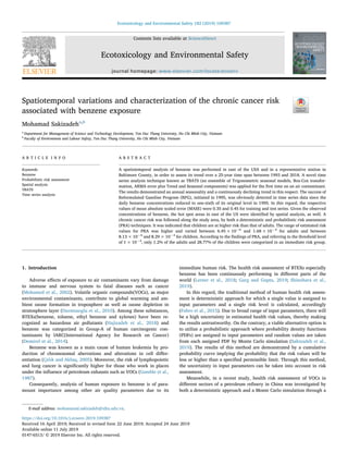
4. enough evidence about the suitability of this distribution.
The mean and standard deviation of lognormal model using a
bootstrap simulation were −5.413 and 0.414 which are very close to
the values obtained in Table 1. Moreover, the 95% percentile of con-
fidence interval for the mean varied from −5.506 to −5.319 while that
of standard deviation fluctuated between 0.351 and 0.479. The final
density plot, cumulative distribution function plot, quantile-quantile
plot (q-q plot) and probability-probability plot (p-p plot) of lognormal
model versus that of empirical data have been depicted in Fig. 3S. This
graph gives more evidence about the suitability of lognormal model for
the data of interest.
On the other hand, the frequency distribution along with cumula-
tive probability plot of deterministic and probabilistic health risk as-
sessment methods have been given in Fig. 1. According to the results,
children are at higher risk than that of adults with respect to the
findings of both methods. Considering the threshold of World Health
Organization(WHO), life time cancer risk values between 1 × 10−6
and
1 × 10−5
are categorized as acceptable while for risk values exceeding
1 × 10−4
, an action is required (Legay et al., 2011; Demirel et al.,
2014). These threshold levels were shown by green, blue and red lines
in Fig. 1. Given the findings of deterministic approach for adults, all of
the estimated cancer risk values exceeded 1 × 10−5
whereas only 1.3%
of calculated risk values were higher than 1 × 10−4
. As a whole, the
estimated risk valued fluctuated between 1.17 × 10−5
and
1.17 × 10−4
. The first and third quantile risk values were 2.03 × 10−5
and 3.55 × 10−5
with a median of 2.71 × 10−5
. On the contrary, about
14.5% of the estimated cancer risks passed the cutoff level of 1 × 10−4
while all of the calculated levels were higher than the acceptable
threshold of 1 × 10−5
. In summary, the risk values worked out for the
children varied between 2.73 × 10−5
and 2.73 × 10−4
with a median
of 6.29 × 10−5
. In this regard, the associated first and third quantiles
were 4.69 × 10−5
and 8.23 × 10−5
, accordingly.
Although, there have been multiple researches related to health risk
assessment of VOCs and especially benzene however, given the large
physical extent of the study area (1,598,576 km2
), few researches were
performed on such a large extent. In one of related recent studies,
Dimitriou and Kassomenos (2019) estimated the cancer health risk due
to inhalation of benzene in 11 European countries using only one
sample from each respective country. It was found that the lifetime
cancer risks associated with all of the countries were higher than the
threshold value of 1 × 10−6
; a finding that was consistent with the
results of the current research. In addition, in nine out of eleven sta-
tions, the estimated risk values were higher than 1 × 10−5
for adults.
There was not any report about the risk values of benzene for children
in the later study. In another study, cancer risk levels of benzene were
calculated for the state of Florida in the USA using the data of 23
Fig. 1. Frequency distribution and cumulative probability plots of deterministic (top) and probabilistic (bottom) health risk assessment methods applied on benzene
concentrations.
M. Sakizadeh Ecotoxicology and Environmental Safety 182 (2019) 109387
4

5. monitoring stations. It was found that the cancer risk values varied
between 4.56 × 10−6
and 8.93 × 10−5
(Johnson et al., 2009). The
lower estimated risk of this state was probably due to the lower de-
tected benzene values, fluctuating between 0.18 ppb and 3.58 ppb
compared to 0.58 ppb and 5.80 ppb in the current research. In another
similar study on 227 outdoor sites in southeast Michigan, 5% of the
samples exceeded the permissible level of 1 × 10−4
(Jia et al., 2008).
It should be noted that the calculated risk values in this study are
related to outdoor samples whereas the indoor values of benzene were
possibly higher as was mentioned in earlier researches(Guo et al., 2004;
Massolo et al., 2010) so, the actual risk values for indoor inhalation may
be higher, accordingly. Moreover, as the level of industrialization in-
crease, the health risk due to benzene will rise and vice versa. For in-
stance, the detected outdoor levels of VOCs including benzene in La
Plata, Buenos Aires (Argentine) in industrial areas were between three
and six times higher than that of other regions (Massolo et al., 2010).
Other factors such as smoking in indoor places may also exacerbate the
condition since one of the major sources of benzene in indoor places is
smoking (Demirel et al., 2014). The highest estimated lifetime cancer
risk values of benzene based on a literature review conducted by the
author of this paper was 1.05 × 10−3
in Argentina and related to gas
stations (Lerner et al., 2012) while values as high as 1.1 × 10−2
were
also observed for rotary incinerator workshops in China (An et al.,
2014). These risk values are significantly higher than those found in the
current study.
Despite the fact that calculated values of the cancer risk by de-
terministic approach seem to be reliable and it is the dominant method
in environmental and public health researches but there are high un-
certainties in some input parameters such as body weight and inhala-
tion rate as was shown in earlier studies (Guo et al., 2004; Dimitriou
and Kassomenos, 2019). That is why a probabilistic method was also
followed in the current research to take these uncertainties into account
in estimated risk levels.
Meanwhile, as was expected, the range of estimated risk values for
PRA was higher and varied between 6.45 × 10−6
and 1.68 × 10−4
for
the adults and between 8.13 × 10−6
and 8.29 × 10−4
for the children.
There are some sources of uncertainties inherent in human health risk
assessment. In this study, it was tried to take the uncertainties asso-
ciated with human body weight, concentration of benzene in ambient
air, inhalation rate and exposure duration into account in the prob-
abilistic method. However, the results may still be uncertain due to
other parameters such as cancer slope factor which is estimated through
either occupational studies or toxicological researches in animals
(Zhang et al., 2018a, b). This parameter has to be fixed at its default
level in risk estimation though.
In the current research, the estimated median cancer risk for adults
was 3.41 × 10−5
and its first and third quantiles ranged from
2.48 × 10−5
to 4.68 × 10−5
. Moreover, the median value for the
children was higher and equal to 6.92 × 10−5
whereas the respective
values of the first and third quantiles fluctuated between 4.44 × 10−5
and 1.07 × 10−4
. In contrast to the deterministic approach, 99.5% of
the calculated cancer risk levels for the adults and 99.95% for the
children were higher than 1 × 10−5
. Referring to the threshold level of
1 × 10−4
, only 1.2% of the adults and 28.77% of the children were
categorized in an immediate risk group.
The redeeming features of PRA approach over that of deterministic
method were discussed in other published literature and the reader can
refer to them for further information (e.g.Richardson, 1996; Thompson
and Graham, 1996). In this context, there are two major advantages
associated with PRA versus that of deterministic method. Firstly, since
the distribution of resultant risk or exposure across the population of
interest is created through PRA so, the proportion of people for which
the estimated risk exceeds a specified reference dose can also be cal-
culated accordingly. In contrast, in the former technique (e.g. de-
terministic approach), we can only specify whether or not the estimated
risk level pass a permissible limit (Richardson, 1996). It can be assumed
that 30% of a population exceeds a reference dose but its respective risk
value falls below the threshold level. The other main advantage of PRA
is the possibility of defining risk management scenarios for population
exposure. For instance, what would be the amount of risk if we reduce
the ambient benzene level to half of its current concentration by
adopting pollution control strategies?
Despite of numerous studies on deterministic approach for benzene
and other VOCs, the number of probabilistic researches is not that much
high. For instance, in one of the example studies in South Korea, the
proportion of the population with cancer risk values exceeding the
threshold level of 1 × 10−6
varied from 87% to 98% whereas those
passing the cut-off level of 1 × 10−5
fluctuated between 1% and 8%
among three considered sites (Choi et al., 2011). The main difference of
the current research and the latest one was assignment of PDFs for
exposure duration and concentration of benzene in addition to inhala-
tion rate and body weight. In another probabilistic approach conducted
in Turkey for risk assessment of benzene, only 30% of the population of
interest exceeded the permissible level of 1 × 10−6
(Sofuoglu et al.,
2011) which is significantly lower than the findings of the current re-
search.
In contrast, considering spatial analysis of benzene, the results of
10-fold cross-validation with respect to different performance metrics
have been rendered in Table 2. In this context, the results were more
sensitive to the parameter of inverse distance power (idp) than the
number of nearest observations used for the local predicting (nmax).
Among different values that used for optimization, the best results were
found for an idp of 1 and nmax of 12. The RMSE, which is one of the
most frequent accuracy measures in environmental sciences (Li, 2017),
associated with these parameters was 0.519 however one of the dis-
advantages of this metric is its dependency to the scale of target vari-
able. On the contrary, the values of RMAE next to RRMSE are in-
dependent of the scale/unit of samples and do not change with the
mean of sample values as well. The values of these respective metrics
were 29.80% and 47.21% for RMAE and RRMSE. The final criteria used
in this study were VEcv and E1 which are reliable tools to measure the
accuracy of models(Li, 2016) and do not change with the variance of
data in addition to containing the redeeming features of RMAE and
RRMSE(Li, 2017). The VEcv and E1 found for the best performed model
were 27.73% and 24.20%, respectively.
The map produced by Idw simulation has been illustrated in Fig. 2.
According to the findings; the southeast part of the study area is the
least contaminated region which covers states like Florida, Georgia,
South Carolina, and part of North Carolina. Contrarily, the eastern
states like New Jersey, Pennsylvania, Delaware and part of Virginia,
North Carolina, Maine and Vermont are among the most contaminated
regions. As a whole, there is an increasing trend of contamination as we
move from the west to the east in the central states. In this respect, New
Jersey is the most densely populated US state, though the level of
benzene has declined approximately four times between 1999 and 2009
due to implementation of pollution control programs(Lioy and
Table 2
Cross-validation results of idw spatial method in eastern part of the US.
Optimization parameters Performance criteria
nmax idp RMAE RMSE RRMSE VEcv E1
5 2 30.83 0.53 48.31 24.34 21.58
7 2 30.43 0.52 47.66 26.35 22.63
9 2 30.40 0.52 47.67 26.30 22.68
11 2 30.33 0.52 47.54 26.72 22.85
13 2 30.43 0.52 47.61 26.49 22.61
15 2 30.40 0.52 47.63 26.44 22.70
12 1 29.80 0.52 47.21 27.73 24.20
12 3 30.75 0.53 47.82 25.85 21.81
12 4 31.03 0.53 48.26 24.49 21.09
12 5 31.27 0.54 48.75 22.95 20.48
M. Sakizadeh Ecotoxicology and Environmental Safety 182 (2019) 109387
5

6. Georgopoulos, 2011). Meanwhile, in a study in the latest state, aromatic
VOCs (e.g. BTEXs) including benzene had the highest concentration and
frequency of exposure compared to other volatile chemicals (Harkov
et al., 1984) however due to low degradation rate of this contaminant,
the population exposure to benzene is more significant, accordingly
(Korte and Klein, 1982). The highest concentration of benzene found in
the current study was 3.9 ppb and recorded in Pennsylvania State. In a
recent study in Pennsylvania, it was concluded that a significant level of
ambient benzene is released through natural gas fracking (Meng, 2015).
All in all, this toxic substance can be attributed to both mobile (motor
vehicles) and stationary sources such as petroleum refinery (Hsu et al.,
2018), petrol stations (Hazrati et al., 2016) and oil exploration (Nance
et al., 2016) in addition to tobacco smoking in indoor places (Wallace,
1989).
3.2. Temporal variations of benzene
The results of multiple seasonal decomposition of benzene in
Baltimore County between 6-1-1993 and 8-31-2018 were illustrated in
Fig. 3. According to this graph, there is only an annual seasonality as-
sociated with the data (the third panel) but its amplitude has steadily
decreased from 1995 onwards. By seasonality, it means a periodic
pattern of either decrease or increase (e.g. over month, quarter or year),
that occurs between years (Naumova, 2006). It is hard to identify the
exact seasonal drivers since a number of factors may be involved in this
respect. However, even though, since several studies have exhibited the
effect of meteorological parameters (such as velocity and direction of
wind, temperature, humidity etc.) on fluctuations of benzene (Liu et al.,
2009; Marć et al., 2015) so, these factors probably made a large con-
tribution on detected seasonality in this study.
Referring to the vertical scales, until 1995, the remainder part (e.g.
residual or error) was more important than trend and seasonal com-
ponents but thereafter the residual part had a relatively narrow range in
comparison with the other components. As it is clear, over the period of
1993–2018, the concentrations of benzene exhibit a declining trend in
the study area in which the daily concentration has reduced to one-sixth
of its original level in 1995 (the second panel). This finding was con-
sistent with previous studies on time series of benzene in other states
(Aleksic et al., 2005; Reiss, 2006). In order to further consider this re-
ducing trend, we have to inspect the time series of original data (top
panel) in Fig. 3. Between 1993 and 1994, the daily mean benzene level
increased dramatically from about 8 ppb to approximately 28 ppb but
since then it slumped to roughly 15 ppb in 1996. This sudden drop was
consistent with implementation of the Reformulated Gasoline Program
Fig. 2. Spatial prediction of benzene (ppb) in eastern states of the US.
M. Sakizadeh Ecotoxicology and Environmental Safety 182 (2019) 109387
6

7. (RFG) in 1995, resulting in production of a more clean gasoline in 17
states of the USA including Maryland and Baltimore County. During the
first phase of this program between 1995 and 1999, 17% reduction in
VOCs emissions from vehicles was achieved (USEPA, 1999). This pro-
gram has been combined with industrial controls so, a substantial de-
crease in the time series can be observed by 2018.
Meanwhile, the TBATS model that applied for time series decom-
position in this study has several different advantages over similar de-
composition techniques. For example, the normalization is not required
for trigonometric terms so, they are more appropriate for time series
decomposition. In addition, the resultant components of seasonal de-
composition are smoother.
On the other hand, by taking the seasonality detected through time
series decomposition into account, a TBATS model was fitted to the
training series followed by its forecast for the test series, for which the
results were rendered in Table 3. According to findings for the test and
training series, there is an over-fitting problem related to the model
suggesting that the out-of-sample forecasting ability of this model is
lower than that of the training series since all of the performance cri-
teria were higher for test data compared to the training set. Considering
the range of daily benzene values, the results found for RMSE and MAE
were satisfactory. Referring to Table 3, the associated RMSE for the
training and test set were 1.05 and 1.07 while that of MAE were 0.53
and 0.67, respectively. The main disadvantage related to RMSE is its
sensitivity to outliers so, MAE may be a more viable metric according to
some researchers (e.g. Armstrong and Forecasting, 2001).
In contract, the most difference between training and test series
associated with each metric was obtained for the mean absolute
Fig. 3. Multiple seasonal decomposition of time series of benzene between 1993 and 2018 in Baltimore County, Maryland, USA.
Table 3
Performance of time series prediction with TBATS model on training and test
set.
RMSE MAE MAPE MASE
Training series 1.05 0.53 19.38 0.35
Test series 1.07 0.68 45.67 0.45
M. Sakizadeh Ecotoxicology and Environmental Safety 182 (2019) 109387
7

8. percentage error (MAPE) with respective values of 19.38% and 45.67%
though its main issue is that a heavier penalty is put on positive errors
than negative ones (Makridakis, 1993). Finally, the most recommended
accuracy measure according to Hyndman and Koehler (2006) is MASE.
In this metric, the scale of data is removed by comparing the obtained
forecasts with a benchmark technique for which naïve method is ap-
plied. A scaled error for which the values of forecasts are better than the
average naïve forecast will result in a MASE of lower than one other-
wise it produces values higher than one (Hyndman and
Athanasopoulos, 2018). In this regard, the respective values of MASE
were 0.35 and 0.45 for training and test series, demonstrating the better
performance of the applied method versus that of naïve approach. As
was mentioned earlier, conventional time series techniques are not able
to handle these kinds of daily series.
The final forecasts were obtained for three seasonal periods by the
TBATS model and the associated result was depicted in Fig. 4. With
respect to the final results, the model selected for the training data was
a TBATS equal to (0.003,{5,5},-,{ < 365,10 > }). It implied that a Box-
Cox parameter of 0.003 has been applied in order to account for non-
linearity in the model which was shown by omega in the original
equation (equation (3)). On the contrary, the residual (error) part was
modeled by an ARMA (5,5). In this case, no damping parameter was
utilized for the model of interest. It means that identical predictions
obtained for short run and long run trends. This finding is consistent
with the annual seasonality exhibited by multi-seasonal decomposition
(Fig. 3) and it seems as if the seasonality has been reproduced well since
the seasonal component has roughly been fixed from 2014 onwards.
Finally, m1 which denotes seasonal periods in equation (3) was 365 in
this case that is in agreement with the finding for multi-seasonal de-
composition too, while a Fourier term of 10 for each seasonality was
also applied.
The model applied in the current research contains numerous re-
deeming features over that of conventional methods which was dis-
cussed. For instance, the time series with double seasonal periods (such
as both annual and weekly), non-integer seasonality (e.g.an annual
seasonality equal to 365.25 or a weekly seasonality of 52.129), high
frequency seasonality (e.g.in hourly time series data) and dual calendar
effect (such as in Islamic nations with both Hejri and Gregorian
Fig. 4. Three seasonal periods of benzene forecasted by TBATS model.
M. Sakizadeh Ecotoxicology and Environmental Safety 182 (2019) 109387
8

9. calendars) cannot be handled with traditional time series modeling
techniques. However, the TBATS model can train and forecast these
cases due to its trigonometric formulation and state space modeling
features. Moreover, classical time series approaches, like exponential
smoothing, assume that the model residuals (errors) are serially un-
correlated and thus under violation of this underlying assumption, the
modeling results may not be valid. In contrast, using TBATS approach,
not only the possibility of serial autocorrelation of residuals can be
taken into account but also the time series with nonlinear features can
be trained through inclusion of Fourier series in modeling process.
The only downside associated with the predictions obtained in this
study is that 80% and 95% intervals were too wide; a prevalent problem
with TBATS models as mentioned by Hyndman and Athanasopoulos
(2018). It shows that there are high uncertainties related to out-of-
sample predictions in a way, as the time progresses, the forecast in-
tervals tend to widen. It should be noted that following estimation of
model parameters like smoothing, damping and Box-Cox transforma-
tion plus ARMA coefficients; the point forecasts and prediction intervals
can be obtained during the forecasting process using the inverse of Box-
Cox transformation. However, this interval is monotonically increasing
so that the required probability coverage is retained for the forecast
intervals. The high forecast intervals obtained in this study are in
agreement with that of Brozyna et al. (2018) using TBATS model where
the confidence interval of forecasts for daily demand of electric energy
were more than double higher than those of monthly data.
This study was the first application of TBATS model for daily time
series prediction of an air contaminant. There were some earlier suc-
cessful applications of this technique in environmental epidemiology
Fig. 5. Calendar plot produced for one decade of benzene data in Baltimore County, Maryland.
M. Sakizadeh Ecotoxicology and Environmental Safety 182 (2019) 109387
9

10. (Cherrie et al., 2018), water resources (Barrela et al., 2017) and climate
change research (Tudor, 2016), anyhow. In order to more specifically
consider seasonality of benzene, a calendar plot for one decade of data
was created and has been depicted in Fig. 5. As it is clear, a strong
seasonality is obvious for which the values are lower in January–April
and October–December whereas higher levels of benzene were recorded
in May–September from 1998 to 2007. This seasonality is more obvious
in the first four years and less clear in the following years. It is not easy
to mention the main reasons for this seasonality but as explained earlier
meteorological parameters have possibly made a great contribution in
this respect.
4. Conclusion
In this study, daily time series of a toxic air contaminant (benzene)
was investigated over a 25-year time period. These daily environmental
data series usually contain complicated seasonal patterns such as
monthly, quarterly and annually. By multi-seasonal decomposition of
time series, a continuous declining trend was identified that started
following implementation of Reformulated Gasoline Program (RFG) in
1995. Since conventional methods of time series forecasting such as
ARIMA are unable to handle these higher frequency time series so, an
advanced forecasting method known as TBATS was applied for the time
series of interest. According to the findings of this study, the main
disadvantages of this technique were its low out-of-sample forecasting
ability besides its wide confidence intervals. However even though, this
method is able to decompose complex seasonality and find the suitable
model in a completely automatic process by minimization of AIC,
something that is both time consuming and need enough expert in case
of working with other time series forecasting approaches. The auto-
matic process of this technique is an asset since the numbers of involved
parameters are very high and manually adjusting all of these para-
meters is not an easy task to accomplish. The other subject that was
investigated in this study was chronic cancer risk assessment due to
inhalation of benzene by both deterministic and probabilistic methods.
It was concluded that the children are at higher risk than that of adults
and despite the considerable decrease of benzene which exhibited by
time series analysis, a significant number of inhabitants are still at an
immediate risk. In addition, due to high uncertainty associated with
input parameters, probabilistic technique may be a more realistic
method for health risk assessment than that of deterministic approach.
Acknowledgement
The data used in the current research were results of the collective
efforts of dedicated field crews, laboratory staff, data management and
quality control staff, analysts and many others from EPA, states, tribes,
federal agencies, universities, and other organizations. The author ex-
press his gratitude to all those who contributed to production of these
data. This research did not receive any specific grant from funding
agencies in the public, commercial, or not-for-profit sectors.
Appendix A. Supplementary data
Supplementary data to this article can be found online at https://
doi.org/10.1016/j.ecoenv.2019.109387.
References
Aleksic, N., Boynton, G., Sistla, G., Perry, J., 2005. Concentrations and trends of benzene
in ambient air over New York State during 1990–2003. Atmos. Environ. 39,
7894–7905.
An, T., Huang, Y., Li, G., He, Z., Chen, J., Zhang, C., 2014. Pollution profiles and health
risk assessment of VOCs emitted during e-waste dismantling processes associated
with different dismantling methods. Environ. Int. 73, 186–194.
Armstrong, J.S., Forecasting, P.O., 2001. A Handbook for Researchers and Practitioners.
Kluwer Academic Publishers, MA.
Assaf, H., Saadeh, M., 2009. Geostatistical assessment of groundwater nitrate con-
tamination with reflection on DRASTIC vulnerability assessment: the case of the
Upper Litani Basin, Lebanon. Water Resour. Manag. 23, 775–796.
Barrela, R., Amado, C., Loureiro, D., Mamade, A., 2017. Data reconstruction of flow time
series in water distribution systems–a new method that accommodates multiple
seasonality. J. Hydroinf. 19, 238–250.
Brozyna, J., Mentel, G., Szetela, B., Strielkowski, W., 2018. Multi-seasonality in the
TBATS model using demand for electric energy as a case study. Econ. Comput. Econ.
Cybern. Stud. Res. 52 (1), 229–246.
Çelık, A., Akbaş, E., 2005. Evaluation of sister chromatid exchange and chromosomal
aberration frequencies in peripheral blood lymphocytes of gasoline station atten-
dants. Ecotoxicol. Environ. Saf. 60, 106–112.
Cherrie, M.P., Nichols, G., Iacono, G.L., Sarran, C., Hajat, S., Fleming, L.E., 2018.
Pathogen seasonality and links with weather in England and Wales: a big data time
series analysis. BMC Public Health 18, 1067.
Choi, E., Choi, K., Yi, S.-M., 2011. Non-methane hydrocarbons in the atmosphere of a
Metropolitan City and a background site in South Korea: sources and health risk
potentials. Atmos. Environ. 45, 7563–7573.
D'Agostino, R.B., 1986. Goodness-of-fit-techniques. CRC press.
De Livera, A.M., Hyndman, R.J., Snyder, R.D., 2011. Forecasting time series with complex
seasonal patterns using exponential smoothing. J. Am. Stat. Assoc. 106, 1513–1527.
Demirel, G., Özden, Ö., Döğeroğlu, T., Gaga, E.O., 2014. Personal exposure of primary
school children to BTEX, NO2 and ozone in Eskişehir, Turkey: relationship with in-
door/outdoor concentrations and risk assessment. Sci. Total Environ. 473, 537–548.
Dimitriou, K., Kassomenos, P., 2019. Allocation of excessive cancer risk induced by
benzene inhalation in 11 cities of Europe in atmospheric circulation regimes. Atmos.
Environ. 201, 158–165.
Durmusoglu, E., Taspinar, F., Karademir, A., 2010. Health risk assessment of BTEX
emissions in the landfill environment. J. Hazard Mater. 176, 870–877.
Efron, B., Tibshirani, R.J., 1994. An Introduction to the Bootstrap. CRC press.
Fabro, A.Y.R., Ávila, J.G.P., Alberich, M.V.E., Sansores, S.A.C., Camargo-Valero, M.A.,
2015. Spatial distribution of nitrate health risk associated with groundwater use as
drinking water in Merida, Mexico. Appl. Geogr. 65, 49–57.
Gamble, J., Jones, W., Minshall, S., 1987. Epidemiological-environmental study of diesel
bus garage workers: acute effects of NO2 and respirable particulate on the respiratory
system. Environ. Res. 42, 201–214.
Gardner Jr., E.S., McKenzie, E., 1985. Forecasting trends in time series. Manag. Sci. 31,
1237–1246.
Garg, A., Gupta, N., 2019. A comprehensive study on spatio-temporal distribution, health
risk assessment and ozone formation potential of BTEX emissions in ambient air of
Delhi, India. Sci. Total Environ. 659, 1090–1099.
Guo, H., Lee, S., Chan, L., Li, W., 2004. Risk assessment of exposure to volatile organic
compounds in different indoor environments. Environ. Res. 94, 57–66.
Hajizadeh, Y., Mokhtari, M., Faraji, M., Mohammadi, A., Nemati, S., Ghanbari, R.,
Abdolahnejad, A., Fard, R.F., Nikoonahad, A., Jafari, N., 2018. Trends of BTEX in the
central urban area of Iran: a preliminary study of photochemical ozone pollution and
health risk assessment. Atmos. Pollut. Res. 9, 220–229.
Han, Y., Jiang, P., Dong, T., Ding, X., Chen, T., Villanger, G.D., Aase, H., Huang, L., Xia,
Y., 2018. Maternal air pollution exposure and preterm birth in Wuxi, China: effect
modification by maternal age. Ecotoxicol. Environ. Saf. 157, 457–462.
Harkov, R., Kebbekus, B., Bozzelli, J.W., Lioy, P.J., Daisey, J., 1984. Comparison of se-
lected volatile organic compounds during the summer and winter at urban sites in
New Jersey. Sci. Total Environ. 38, 259–274.
Harper, M., 2000. Sorbent trapping of volatile organic compounds from air. J.
Chromatogr. A 885, 129–151.
Hazrati, S., Rostami, R., Fazlzadeh, M., Pourfarzi, F., 2016. Benzene, toluene, ethylben-
zene and xylene concentrations in atmospheric ambient air of gasoline and CNG
refueling stations. Air Quality, Atmosphere & Health 9, 403–409.
Hsu, C.-Y., Chiang, H.-C., Shie, R.-H., Ku, C.-H., Lin, T.-Y., Chen, M.-J., Chen, N.-T., Chen,
Y.-C., 2018. Ambient VOCs in residential areas near a large-scale petrochemical
complex: spatiotemporal variation, source apportionment and health risk. Environ.
Pollut. 240, 95–104.
Hyndman, R.J., Athanasopoulos, G., 2018. Forecasting: principles and practice. OTexts.
Hyndman, R., Athanasopoulos, G., Bergmeir, C., Caceres, G., Chhay, L., O'Hara-Wild, M.,
Petropoulos, F., Razbash, S., Wang, E., Yasmeen, F., 2019. Forecast: Forecasting
Functions for Time Series and Linear Models. R Package Version 8.5. http://pkg.
robjhyndman.com/forecast.
Hyndman, R.J., Koehler, A.B., 2006. Another look at measures of forecast accuracy. Int. J.
Forecast. 22, 679–688.
Jia, C., Batterman, S., Godwin, C., 2008. VOCs in industrial, urban and suburban
neighborhoods, Part 1: indoor and outdoor concentrations, variation, and risk dri-
vers. Atmos. Environ. 42, 2083–2100.
Johnson, G.T., Harbison, S.C., McCluskey, J.D., Harbison, R.D., 2009. Characterization of
cancer risk from airborne benzene exposure. Regul. Toxicol. Pharmacol. 55, 361–366.
Korte, F., Klein, W., 1982. Degradation of benzene in the environment. Ecotoxicol.
Environ. Saf (United States) 6.
Kumar, U., Jain, V., 2010. ARIMA forecasting of ambient air pollutants (O 3, NO, NO 2
and CO). Stoch. Environ. Res. Risk Assess. 24, 751–760.
Legay, C., Rodriguez, M.J., Sadiq, R., Sérodes, J.B., Levallois, P., Proulx, F., 2011. Spatial
variations of human health risk associated with exposure to chlorination by-products
occurring in drinking water. J. Environ. Manag. 92, 892–901.
Lerner, J.C., Sanchez, E., Sambeth, J., Porta, A., 2012. Characterization and health risk
assessment of VOCs in occupational environments in Buenos Aires, Argentina. Atmos.
Environ. 55, 440–447.
Lerner, J.E.C., de los Angeles Gutierrez, M., Mellado, D., Giuliani, D., Massolo, L.,
Sanchez, E.Y., Porta, A., 2018. Characterization and cancer risk assessment of VOCs
M. Sakizadeh Ecotoxicology and Environmental Safety 182 (2019) 109387
10

11. in home and school environments in gran La Plata, Argentina. Environ. Sci. Pollut.
Control Ser. 25, 10039–10048.
Li, J., 2016. Assessing spatial predictive models in the environmental sciences: accuracy
measures, data variation and variance explained. Environ. Model. Softw 80, 1–8.
Li, J., 2017. Assessing the accuracy of predictive models for numerical data: not r nor r2
,
why not? Then what? PLoS One 12 e0183250.
Li, J., Zhou, Y., Simayi, M., Deng, Y., Xie, S., 2019. Spatial-temporal variations and re-
duction potentials of volatile organic compound emissions from the coking industry
in China. J. Clean. Prod. 214, 224–235.
Lim, G.Q., Matin, M., John, K., 2019. Spatial and temporal characteristics of ambient
atmospheric hydrocarbons in an active shale gas region in North Texas. Sci. Total
Environ. 656, 347–363.
Lin, W., Wu, K., Lao, Z., Hu, W., Lin, B., Li, Y., Fan, H., Hu, J., 2019. Assessment of trace
metal contamination and ecological risk in the forest ecosystem of dexing mining
area in northeast Jiangxi Province, China. Ecotoxicol. Environ. Saf. 167, 76–82.
Lioy, P.J., Georgopoulos, P.G., 2011. New Jersey: a case study of the reduction in urban
and suburban air pollution from the 1950s to 2010. Environ. Health Perspect. 119,
1351–1355.
Liu, H., Liao, J., Jiang, Y., Zhang, B., Yu, H., Kang, J., Hu, C., Li, Y., Xu, S., 2019. Maternal
exposure to fine particulate matter and the risk of fetal distress. Ecotoxicol. Environ.
Saf. 170, 253–258.
Liu, J., Mu, Y., Zhang, Y., Zhang, Z., Wang, X., Liu, Y., Sun, Z., 2009. Atmospheric levels
of BTEX compounds during the 2008 Olympic Games in the urban area of Beijing. Sci.
Total Environ. 408, 109–116.
Makridakis, S., 1993. Accuracy measures: theoretical and practical concerns. Int. J.
Forecast. 9, 527–529.
Marć, M., Bielawska, M., Wardencki, W., Namieśnik, J., Zabiegała, B., 2015. The influ-
ence of meteorological conditions and anthropogenic activities on the seasonal
fluctuations of BTEX in the urban air of the Hanseatic city of Gdansk, Poland.
Environ. Sci. Pollut. Control Ser. 22, 11940–11954.
Massolo, L., Rehwagen, M., Porta, A., Ronco, A., Herbarth, O., Mueller, A., 2010.
Indoor–outdoor distribution and risk assessment of volatile organic compounds in the
atmosphere of industrial and urban areas. Environ. Toxicol. 25, 339–349.
Meng, Q., 2015. Spatial analysis of environment and population at risk of natural gas
fracking in the state of Pennsylvania, USA. Sci. Total Environ. 515, 198–206.
Mohamed, M.F., Kang, D., Aneja, V.P., 2002. Volatile organic compounds in some urban
locations in United States. Chemosphere 47, 863–882.
Nance, E., King, D., Wright, B., Bullard, R.D., 2016. Ambient air concentrations exceeded
health-based standards for fine particulate matter and benzene during the Deepwater
horizon oil spill. J. Air Waste Manag. Assoc. 66, 224–236.
Naumova, E.N., 2006. Mystery of seasonality: getting the rhythm of nature. J. Public
Health Policy 27, 2–12.
Parra, M., González, L., Elustondo, D., Garrigó, J., Bermejo, R., Santamaría, J., 2006.
Spatial and temporal trends of volatile organic compounds (VOC) in a rural area of
northern Spain. Sci. Total Environ. 370, 157–167.
Reiss, R., 2006. Temporal trends and weekend–weekday differences for benzene and 1, 3-
butadiene in Houston, Texas. Atmos. Environ. Times 40, 4711–4724.
Richardson, G.M., 1996. Deterministic versus probabilistic risk assessment: strengths and
weaknesses in a regulatory context. Hum. Ecol. Risk Assess. Int. J. 2, 44–54.
Sakizadeh, M., Ahmadpour, E., Sharafabadi, F.M., 2019. Spatial analysis of chromium in
southwestern part of Iran: probabilistic health risk and multivariate global sensitivity
analysis. Environ. Geochem. Health 1–16.
Samaniego, F.J., 2014. Stochastic Modeling and Mathematical Statistics: A Text for
Statisticians and Quantitative Scientists. Chapman and Hall/CRC.
Shinohara, N., Okazaki, Y., Mizukoshi, A., Wakamatsu, S., 2019. Exposure to benzene,
toluene, ethylbenzene, xylene, formaldehyde, and acetaldehyde in and around gas
stations in Japan. Chemosphere.
Sofuoglu, S.C., Aslan, G., Inal, F., Sofuoglu, A., 2011. An assessment of indoor air con-
centrations and health risks of volatile organic compounds in three primary schools.
Int. J. Hyg Environ. Health 214, 36–46.
Thompson, K.M., Graham, J.D., 1996. Going beyond the single number: using probabil-
istic risk assessment to improve risk management. Hum. Ecol. Risk Assess. Int. J. 2,
1008–1034.
Tudor, C., 2016. Predicting the evolution of CO2 emissions in Bahrain with automated
forecasting methods. Sustainability 8, 923.
USEPA, 1989. Risk Assessment Guidance for Superfund, vol. 1 Human Health Evaluation
Manuel, Washington, D.C EPA/540/1-89/002.
USEPA, 1994. Methods for Derivation of Inhalation Reference Concentrations and
Application of Inhalation Dosimetry. Office of Health and Environmental Assessment,
Environmental Criteria and Assessment Office, Research Triangle Park, NC EPA/600/
8- 90/066F.
USEPA, 1998. Integrated Risk Information System. available at: https://www.epa.gov/
iris.
USEPA, 1999. Phase II Reformulated Gasoline: the Next Major Step towards Cleaner Air.
EPA/420-F99-024.
USEPA, 2005. National Emissions Inventory. http://www.epa.gov/ttn/chief/net/
2005inventory.html#inventorydata.
Wallace, L.A., 1989. Major sources of benzene exposure. Environ. Health Perspect. 82,
165–169.
Wang, P., Zhang, H., Qin, Z., Zhang, G., 2017. A novel hybrid-Garch model based on
ARIMA and SVM for PM2. 5 concentrations forecasting. Atmos. Pollut. Res. 8,
850–860.
Wu, Z., Han, W., Xie, M., Han, M., Li, Y., Wang, Y., 2019. Occurrence and distribution of
polybrominated diphenyl ethers in soils from an e-waste recycling area in northern
China. Ecotoxicol. Environ. Saf. 167, 467–475.
Yaghmaien, K., Hadei, M., Hopke, P., Gharibzadeh, S., Kermani, M., Yarahmadi, M.,
Emam, B., Shahsavani, A., 2019. Comparative health risk assessment of BTEX ex-
posures from landfills, composting units, and leachate treatment plants. Air Quality,
Atmosphere & Health 1–9.
Zhang, L., Lin, J., Qiu, R., Hu, X., Zhang, H., Chen, Q., Tan, H., Lin, D., Wang, J., 2018a.
Trend analysis and forecast of PM2. 5 in Fuzhou, China using the ARIMA model. Ecol.
Indicat. 95, 702–710.
Zhang, Z., Yan, X., Gao, F., Thai, P., Wang, H., Chen, D., Zhou, L., Gong, D., Li, Q.,
Morawska, L., 2018b. Emission and health risk assessment of volatile organic com-
pounds in various processes of a petroleum refinery in the Pearl River Delta, China.
Environ. Pollut. 238, 452–461.
M. Sakizadeh Ecotoxicology and Environmental Safety 182 (2019) 109387
11