Numerical Method TEP

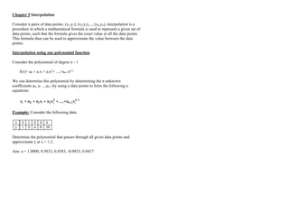
1. Chapter 5 Interpolation
Consider n pairs of data points: (x1,y1), (x2,y2),..., (xn,yn), interpolation is a
procedure in which a mathematical formula is used to represent a given set of
data points, such that the formula gives the exact value at all the data points.
This formula then can be used to approximate the value between the data
points.
Interpolation using one polynomial function
Consider the polynomial of degree n - 1
f(x)= a0 + a1x + a2x2
+ ...,+an-1xn-1
We can determine this polynomial by determining the n unknown
coefficients a0, a1 ...,an-1 by using n data points to form the following n
equations:
1
-
n
i
1
-
n
2
i
2
i
1
0
i x
...,+a
+
x
a
+
x
a
+
a
=
y
Example: Consider the following data.
Determine the polynomial that passes through all given data points and
approximate y at x = 1.3.
Ans: a = 1.0000, 0.5833, 0.4583, -0.0833, 0.0417

2. Lagrange Interpolating Polynomial
For n data points: (x1,y1), (x2,y2),..., (xn,yn), the Lagrange interpolating
polynomial of order n -1 is in the form



n
1
i
i
i(x)y
L
f(x)
Where 













n
1
j
1,
j j
i
j
i
x
x
x
x
(x)
L is the Lagrange function.
For n = 1 (use 2 data points)
x y
x1 y1
x2 y2
For n = 2 (use 3 data points)
x y
x1 y1
x2 y2
x3 y3
For n = 3 (use 4 data points)
x y
x1 y1
x2 y2
x3 y3
x4 y4
f(x) = L1(x)y1 + L2(x)y2
1
2
1
2
2
1
2
1
x
x
x
x
(x)
L
x
x
x
x
(x)
L






f(x) = L1(x)y1 + L2(x)y2 + L3(x)y3
)
x
(x
)
x
(x
)
x
(x
)
x
(x
(x)
L
)
x
(x
)
x
(x
)
x
(x
)
x
(x
(x)
L
)
x
(x
)
x
(x
)
x
(x
)
x
(x
(x)
L
2
3
1
3
2
1
3
3
2
1
2
3
1
2
3
1
2
1
3
2
1















f(x) = L1(x)y1 + L2(x)y2 + L3(x)y3 + L4(x)y4
)
x
(x
)
x
(x
)
x
(x
)
x
(x
)
x
(x
)
x
(x
(x)
L
)
x
(x
)
x
(x
)
x
(x
)
x
(x
)
x
(x
)
x
(x
(x)
L
)
x
(x
)
x
(x
)
x
(x
)
x
(x
)
x
(x
)
x
(x
(x)
L
)
x
(x
)
x
(x
)
x
(x
)
x
(x
)
x
(x
)
x
(x
(x)
L
3
4
2
4
1
4
3
2
1
4
4
3
2
3
1
3
4
2
1
3
4
2
3
2
1
2
4
3
1
2
4
1
3
1
2
1
4
3
2
1





























3. Example: Consider the following data points.
Construct the Lagrange polynomials of order 1 by using the two data points
and order two by using all three data points. Then approximate the value of y
for x = 2 by using the Lagrange polynomials of order 1 and 2.

4. Example: Construct the Lagrange polynomial for the function f(x)= sin(3x)
by using the following data in the table and use it to approximate f(1.5)

5. Newton’s Interpolating Polynomials
)
x
)...(x
x
)(x
x
(x
a
...
)
x
)(x
x
(x
a
)
x
(x
a
a
)
x
(x
a
f(x) 1
n
2
1
n
2
1
3
1
2
1
n
1
i
1
i
1
j
j
i 























  
Divided Difference
j
n
j
1
n
j
1
j
j
n
j
2
j
1
j
n
j
2
j
1
j
j
j
3
j
2
j
1
j
j
3
j
2
j
1
j
3
j
2
j
1
j
j
j
2
j
1
j
j
2
j
1
j
2
j
1
j
j
j
1
j
j
1
j
1
j
j
x
x
]
x
,...,
x
,
f[x
]
x
,...,
x
,
f[x
]
x
,...,
x
,
x
,
f[x
x
x
]
x
,
x
,
f[x
]
x
,
x
,
f[x
]
x
,
x
,
x
,
f[x
x
x
]
x
,
f[x
]
x
,
f[x
]
x
,
x
,
f[x
x
x
y
y
]
x
,
f[x








































]
x
,...,
x
,
x
,
f[x
a
]
x
,
x
,
f[x
a
]
x
,
f[x
a
y
a
n
3
2
1
n
3
2
1
3
2
1
2
1
1





6. Example:
(a) Construct Newton’s interpolation polynomial passing through the following data set.
(b) Let (x, y)=(3, 36) be a new additional data point. Construct Newton’s interpolation polynomial
passing through the following new data set by using (a).
Approximate the value of y when x = 2 by using this Newton’s polynomial.
x y f[xi,xi+1] f[xi,xi+1,xi+2] f[xi,xi+1,xi+2,xi+3] f[xi,xi+1,xi+2,xi+3,xi+4]

7. Example: Determine the Newton’s polynomial that passes through the data points:
and use it to approximate the value of y when x = 3.
x y f[xi,xi+1] f[xi,xi+1,xi+2] f[xi,xi+1,…,xi+3] f[xi,xi+1,…,xi+4] f[xi,xi+1,…,xi+5]