Download to read offline
![Dr.K.Sreenivasa Rao B.Tech, M.Tech, Ph.D VBIT, Hyderabad
1 4 2
2 4 10
3 7 4
4 7 22
5 8 16
6 9 10
> attach(cars)
By using the attach( ) function the database is attached to the R
search path. This means that the database is searched by R when
evaluating a variable, so objects in the database can be accessed by
simply giving their names.
> speed
[1] 4 4 7 7 8 9 10 10 10 11 11 12 12 12 12 13 13 13 13 14 14 14 14
15 15 15 16
[28] 16 17 17 17 18 18 18 18 19 19 19 20 20 20 20 20 22 23 24 24
24 24 25
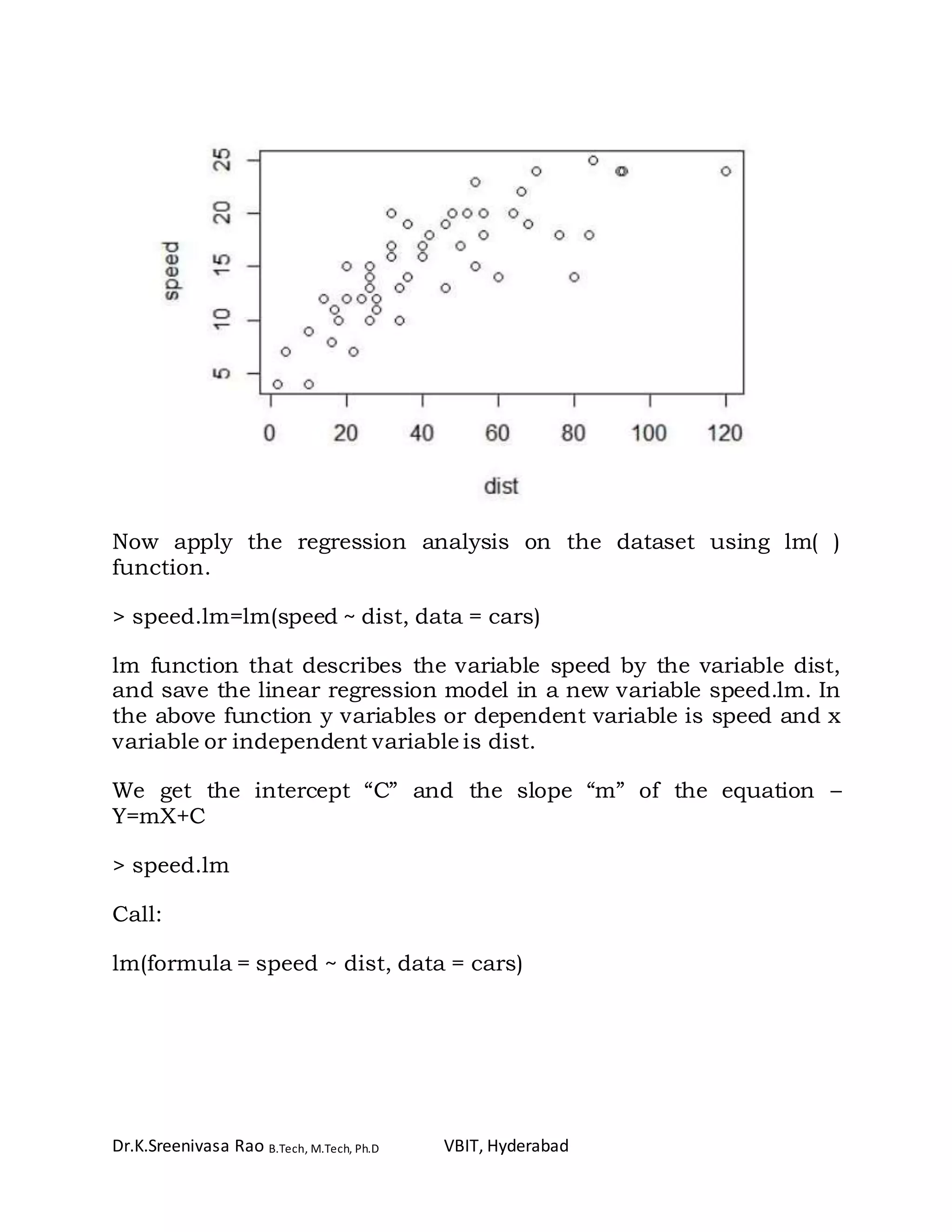
> plot(cars)
> plot(dist,speed)
The plot() function gives a scatterplot whenever we give two numeric
variables.
The first variable listed will be plotted on the horizontal axis.](https://image.slidesharecdn.com/correlationandregressioninr-170506080437/75/Correlation-and-regression-in-r-3-2048.jpg)
![Dr.K.Sreenivasa Rao B.Tech, M.Tech, Ph.D VBIT, Hyderabad
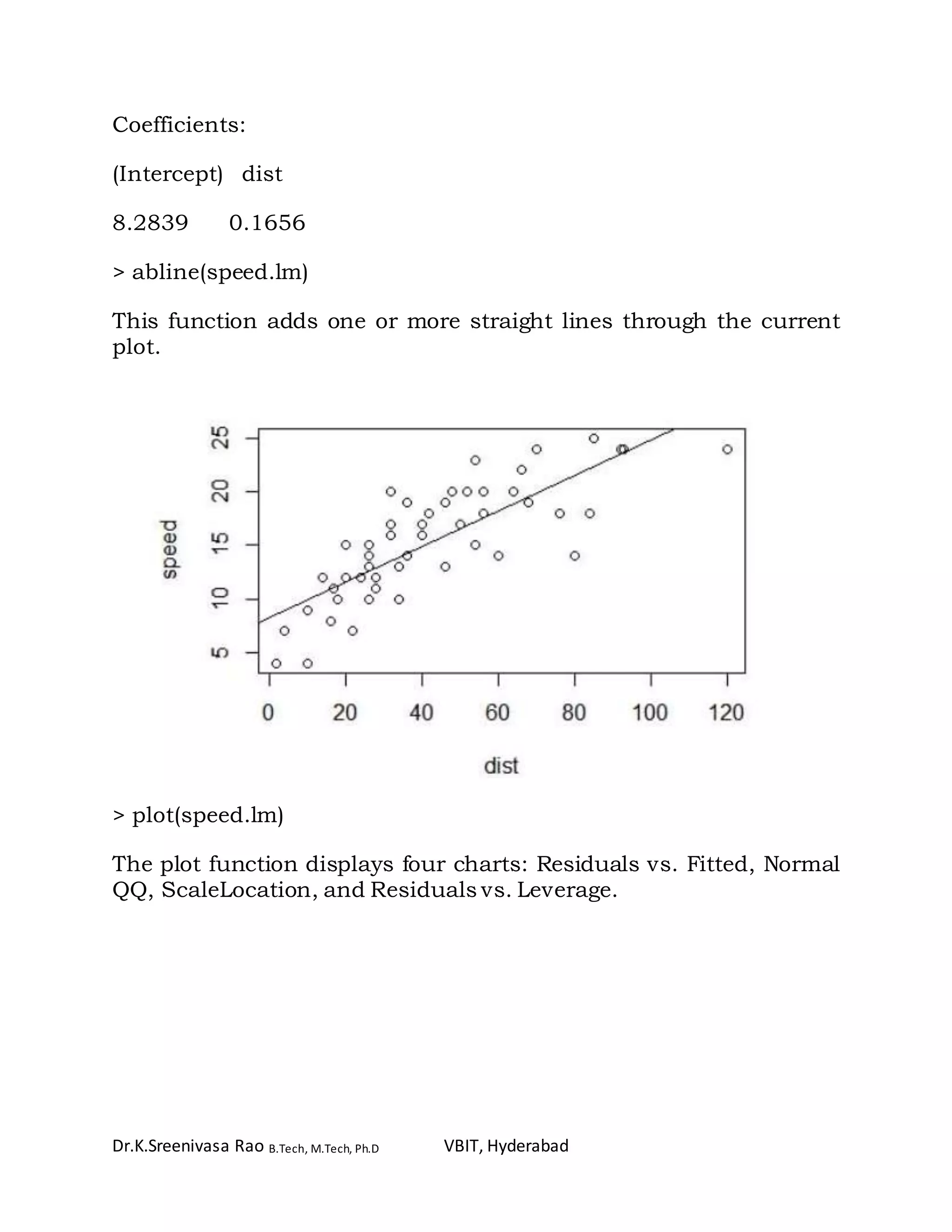
(Intercept) dist
8.2839056 0.1655676
Forecasting/Prediction:
We now fit the speed using the estimated regression equation.
> newdist = 80
> distance = coeffs[1] + coeffs[2]*newdist
> distance
(Intercept)
21.52931
To create a summary of the fitted model:
> summary (speed.lm)
Call:
lm(formula = speed ~ dist, data = cars)
Residuals:
Min 1Q Median 3Q Max
-7.5293 -2.1550 0.3615 2.4377 6.4179
Coefficients:
Estimate Std. Error t value Pr(>|t|)
(Intercept) 8.28391 0.87438 9.474 1.44e-12 ***
dist 0.16557 0.01749 9.464 1.49e-12 ***
---](https://image.slidesharecdn.com/correlationandregressioninr-170506080437/75/Correlation-and-regression-in-r-11-2048.jpg)
![Dr.K.Sreenivasa Rao B.Tech, M.Tech, Ph.D VBIT, Hyderabad
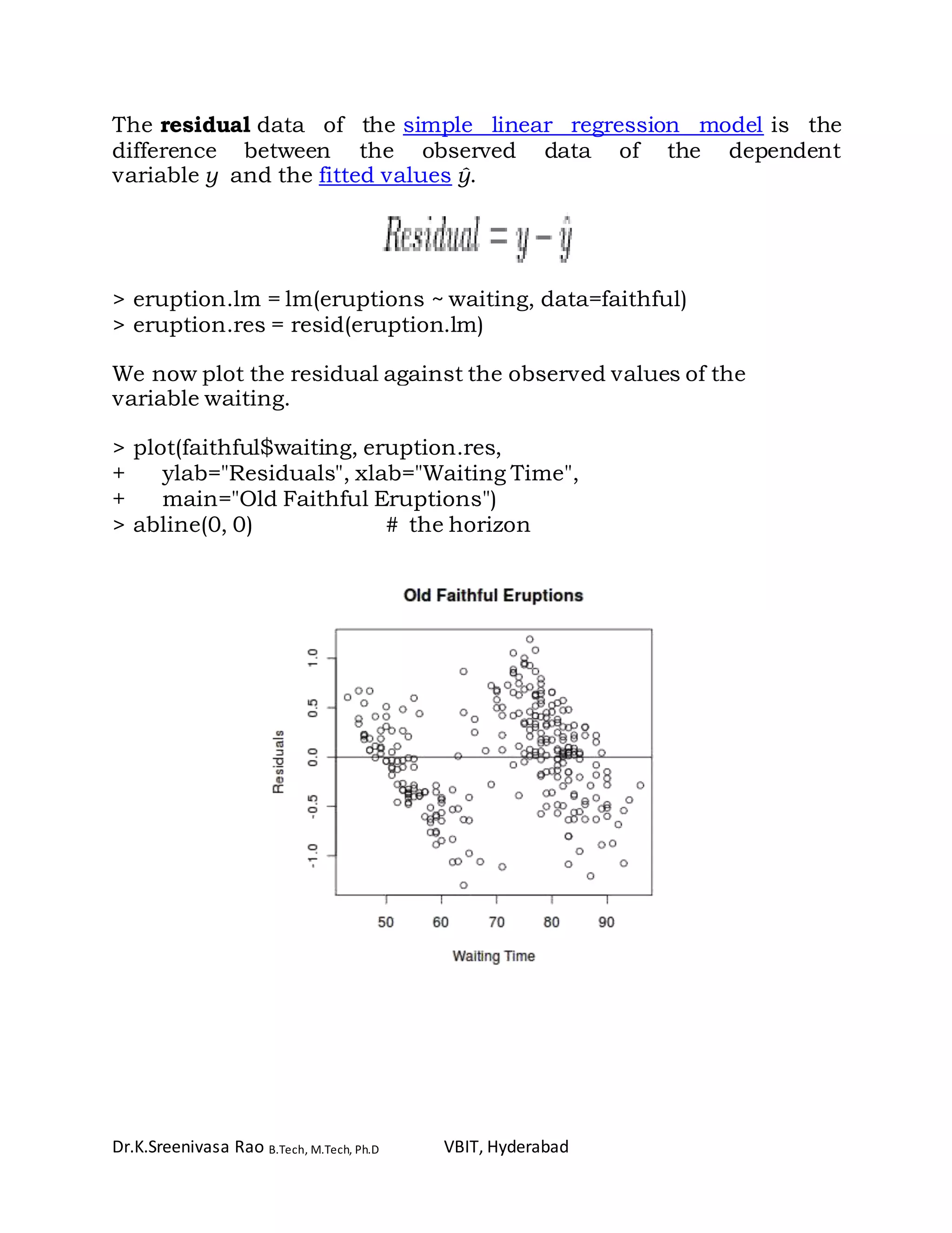
> duration = faithful$eruptions # the eruption durations
> waiting = faithful$waiting # the waiting period
> cov(duration, waiting) # apply the cov function
[1] 13.978
ANOVA:
Analysis of Variance (ANOVA) is a commonly used statistical
technique for investigating data by comparing the means of subsets
of the data. The base case is the one-way ANOVA which is an
extension of two-sample t test for independent groups covering
situations where there are more than two groups being compared.
In one-way ANOVA the data is sub-divided into groups based on a
single classification factor and the standard terminology used to
describe the set of factor levels is treatment even though this might
not always have meaning for the particular application. There is
variation in the measurements taken on the individual components
of the data set and ANOVA investigates whether this variation can
be explained by the grouping introduced by the classification factor.
To investigate these differences we fit the one-way ANOVA model
using the lm function and look at the parameter estimates and
standard errors for the treatment effects.
> anova(speed.lm)
Analysis of Variance Table
Response: speed
Df Sum Sq Mean Sq F value Pr(>F)
dist 1 891.98 891.98 89.567 1.49e-12 ***
Residuals 48 478.02 9.96](https://image.slidesharecdn.com/correlationandregressioninr-170506080437/75/Correlation-and-regression-in-r-16-2048.jpg)
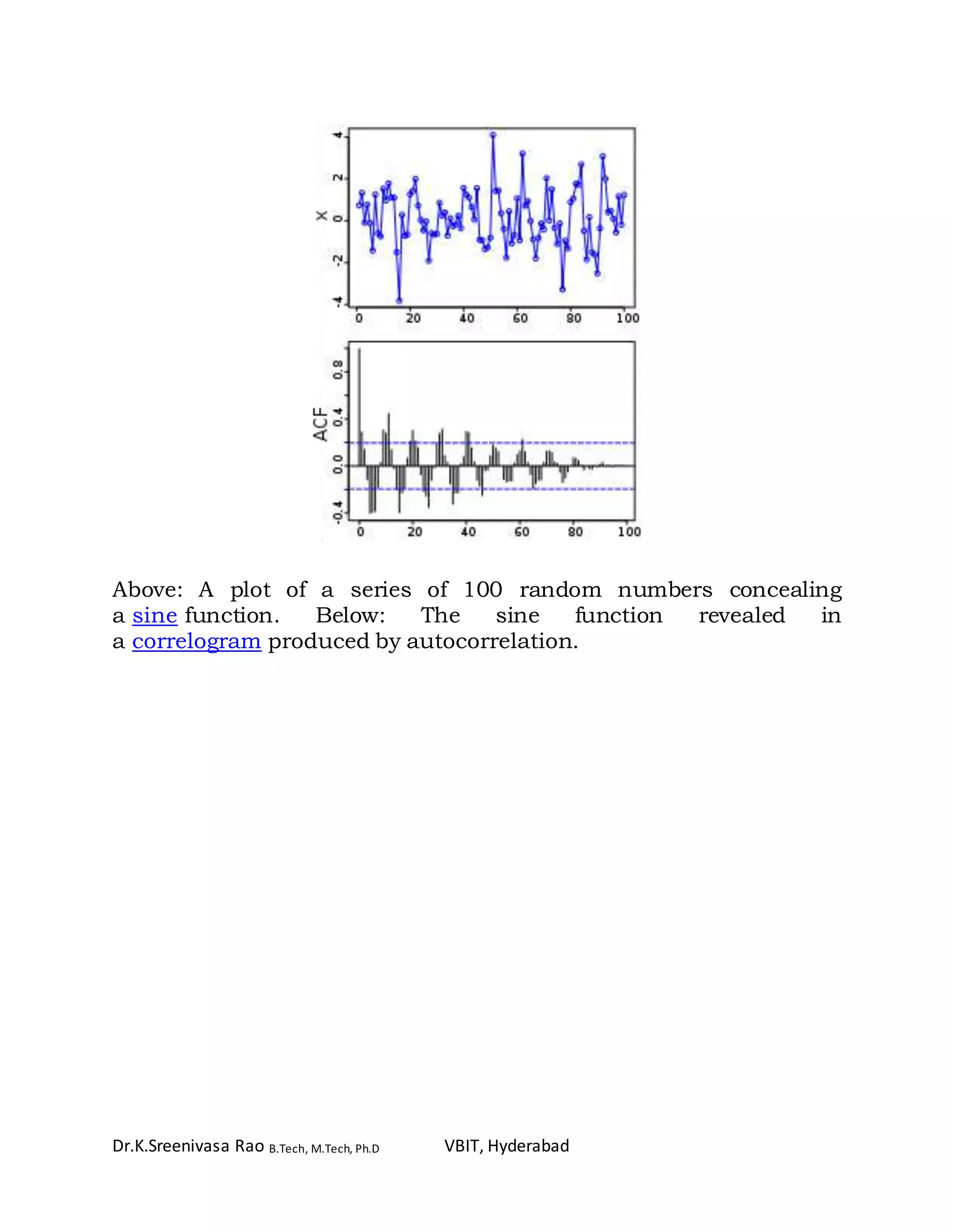
![Dr.K.Sreenivasa Rao B.Tech, M.Tech, Ph.D VBIT, Hyderabad
frequencies. It is often used in signal processing for analyzing
functions or series of values, such as time domain signals.
Autocorrelation is a mathematical representation of the degree of
similarity between a given time series and a lagged version of itself
over successive time intervals.
In statistics, the autocorrelation of a random process is
the correlation between values of the process at different times, as a
function of the two times or of the time lag. Let X be a stochastic
process, and t be any point in time. (t may be an integer for
a discrete-time process or a real number for a continuous-
time process.) Then Xt is the value (or realization) produced by a
given run of the process at time t. Suppose that the process
has mean μt and variance σt
2 at time t, for each t. Then the
definition of the autocorrelation between times s and t is
where "E" is the expected value operator. Note that this expression
is not well-defined for all-time series or processes, because the
mean may not exist, or the variance may be zero (for a constant
process) or infinite (for processes with distribution lacking well-
behaved moments, such as certain types of power law). If the
function R is well-defined, its value must lie in the range [−1, 1],
with 1 indicating perfect correlation and −1 indicating perfect anti-
correlation.](https://image.slidesharecdn.com/correlationandregressioninr-170506080437/75/Correlation-and-regression-in-r-22-2048.jpg)
![Dr.K.Sreenivasa Rao B.Tech, M.Tech, Ph.D VBIT, Hyderabad
(Intercept) UNEM HGRAD
-8255.7511 698.2681 0.9423
> #what is the expected fall enrollment (ROLL) given this year's
unemployment rate (UNEM) of 9% and spring high school
graduating class (HGRAD) of 100,000
> -8255.8 + 698.2 * 9 + 0.9 * 100000
[1] 88028
> #the predicted fall enrollment, given a 9% unemployment rate and
100,000 student spring high school graduating class, is 88,028
students.
> #three predictor model
> #create a linear model using lm(FORMULA, DATAVAR)
> #predict the fall enrollment (ROLL) using the unemployment rate
(UNEM), number of spring high school graduates (HGRAD), and per
capita income (INC)
> threePredictorModel <- lm(ROLL ~ UNEM + HGRAD + INC,
datavar)
> #display model
> threePredictorModel
Call:
lm(formula = ROLL ~ UNEM + HGRAD + INC, data = datavar)
Coefficients:
(Intercept) UNEM HGRAD INC
-9153.2545 450.1245 0.4065 4.2749](https://image.slidesharecdn.com/correlationandregressioninr-170506080437/75/Correlation-and-regression-in-r-28-2048.jpg)

Regression analysis is a predictive modeling technique used to investigate relationships between variables. It allows one to estimate the effects of independent variables on a dependent variable. Regression analysis can be used for forecasting, time series modeling, and determining causal relationships. There are different types of regression depending on the number of variables and the shape of the regression line. Linear regression models the linear relationship between two variables using an equation with parameters estimated to minimize error. Correlation and covariance measures the strength and direction of association between variables. Analysis of variance (ANOVA) compares the means of groups within data. Heteroskedasticity refers to unequal variability of a dependent variable across the range of independent variable values.


![[DSC Europe 25] Dusan Nesic - Securing Tomorrow’s Infrastructure: Why Cyber-P...](https://cdn.slidesharecdn.com/ss_thumbnails/qikbszfftyowjm2q6duw-1-251211083848-8f2ead6b-thumbnail.jpg?width=640&height=640&fit=bounds)


![[DSC Europe 25] Dunja Adzic Jovanovic - AI and Cybersecurity: Defending Data ...](https://cdn.slidesharecdn.com/ss_thumbnails/o1zylpbhrtwnixxq2xj8-7-251211083048-185086f6-thumbnail.jpg?width=640&height=640&fit=bounds)
![[DSC Europe 25] Jon Dajci - Bridging TradFi and DeFi: Building the Future of ...](https://cdn.slidesharecdn.com/ss_thumbnails/fqmhfvlbqhkihjvqvhmu-7-251211083849-6af7e325-thumbnail.jpg?width=640&height=640&fit=bounds)


![[DSC Europe 25] Behzad Hosseini - AI Agents in the Wild: Deploying Models tha...](https://cdn.slidesharecdn.com/ss_thumbnails/3qtejajvsjqrzwfept2c-10-251212103250-7f2b1068-thumbnail.jpg?width=640&height=640&fit=bounds)


