Download to read offline


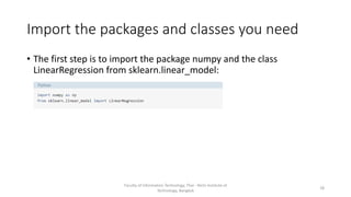
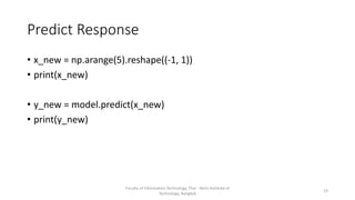
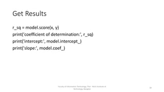
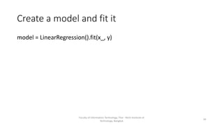
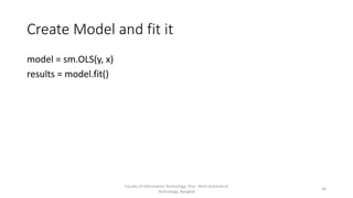
![Get Data
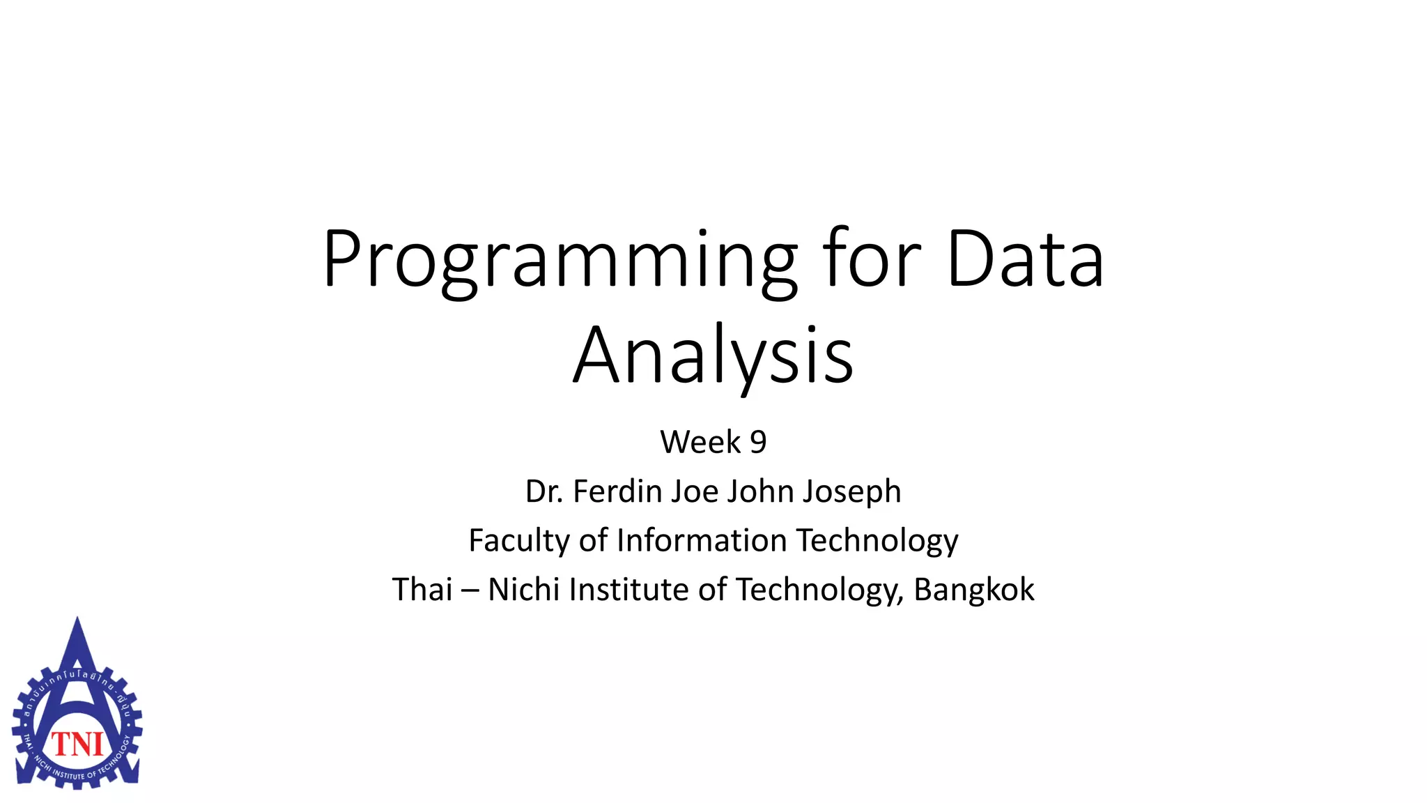
x = [[0, 1], [5, 1], [15, 2], [25, 5], [35, 11], [45, 15], [55, 34], [60, 35]]
y = [4, 5, 20, 14, 32, 22, 38, 43]
x, y = np.array(x), np.array(y)
Faculty of Information Technology, Thai - Nichi Institute of
Technology, Bangkok
26](https://image.slidesharecdn.com/week9-210202094410/85/Week-9-Programming-for-Data-Analysis-26-320.jpg)
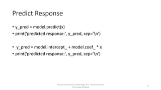
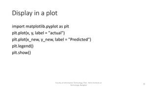
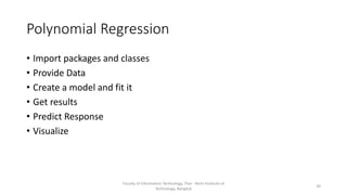
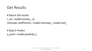
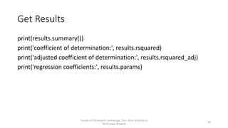
![Predict Response
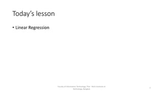
y_pred = model.predict(x)
print('predicted response:', y_pred, sep='n’)
y_pred = model.intercept_ + np.sum(model.coef_ * x, axis=1)
print('predicted response:', y_pred, sep='n’)
y_pred=model.predict(x)
y_pred=model.intercept_+np.sum(model.coef_*x,axis=1)
x_new = [[0, 1], [5, 1], [15, 2], [25, 5], [35, 11], [45, 15], [55, 34], [60,
35]]
y_new = model.predict(x_new)
Faculty of Information Technology, Thai - Nichi Institute of
Technology, Bangkok
29](https://image.slidesharecdn.com/week9-210202094410/85/Week-9-Programming-for-Data-Analysis-29-320.jpg)
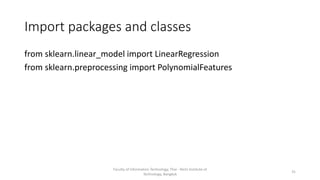
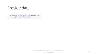
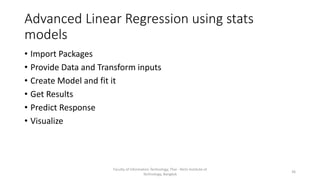
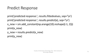
![Provide Data
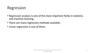
x = np.array([5, 15, 25, 35, 45, 55]).reshape((-1, 1))
y = np.array([15, 11, 2, 8, 25, 32])
Faculty of Information Technology, Thai - Nichi Institute of
Technology, Bangkok
32](https://image.slidesharecdn.com/week9-210202094410/85/Week-9-Programming-for-Data-Analysis-32-320.jpg)
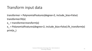
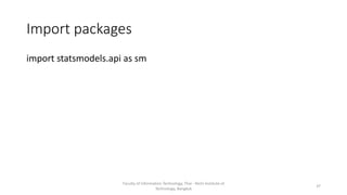
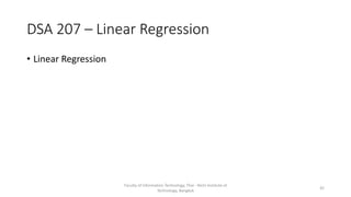
![Provide data and transform inputs
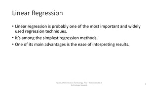
x = [[0, 1], [5, 1], [15, 2], [25, 5], [35, 11], [45, 15], [55, 34], [60, 35]]
y = [4, 5, 20, 14, 32, 22, 38, 43]
x, y = np.array(x), np.array(y)
x = sm.add_constant(x)
Faculty of Information Technology, Thai - Nichi Institute of
Technology, Bangkok
38](https://image.slidesharecdn.com/week9-210202094410/85/Week-9-Programming-for-Data-Analysis-38-320.jpg)

This document discusses different types of linear regression models including simple, multiple, and polynomial linear regression. It provides code examples for implementing linear regression using scikit-learn and statsmodels. Key steps covered include importing packages, providing data, creating and fitting regression models, obtaining results like coefficients and metrics, making predictions on new data, and visualizing models. Types of linear regression covered are simple linear regression with one variable, multiple linear regression with two or more variables, and polynomial regression with higher degree polynomials.