Downloaded 50 times


![LIGHTWAVE Previous Page | Contents | Zoom in | Zoom out | Front Cover | Search Issue | Next Page
111
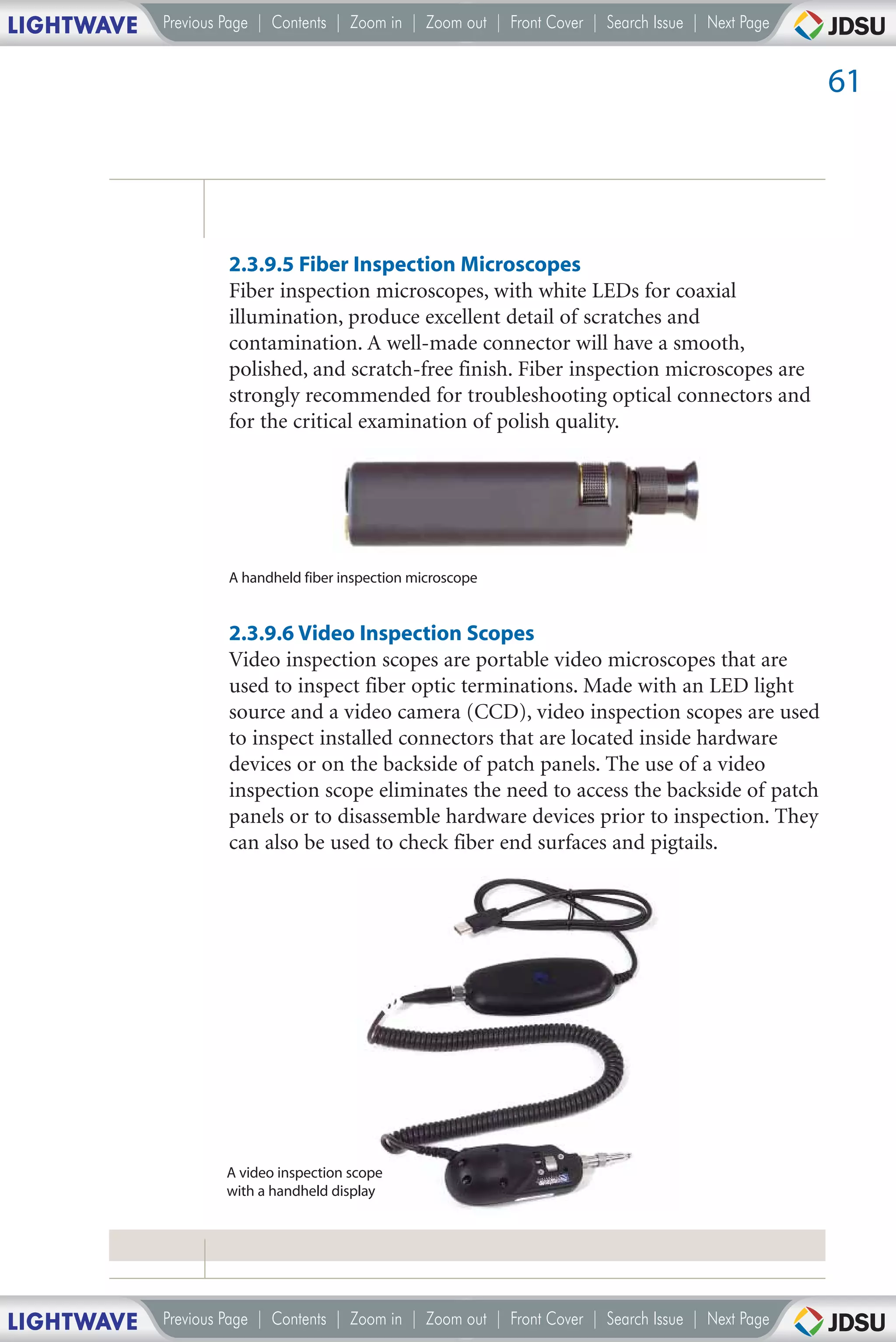
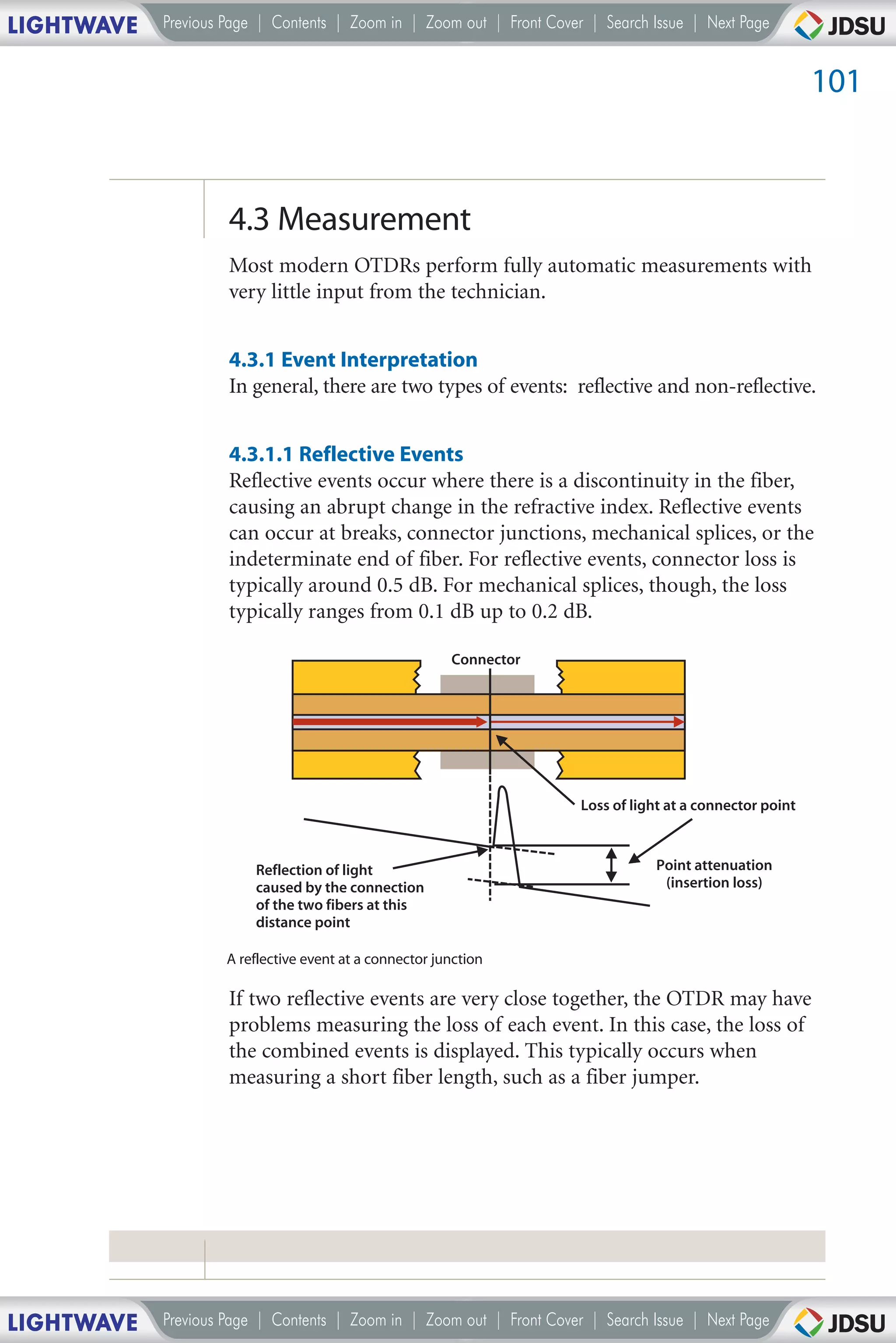
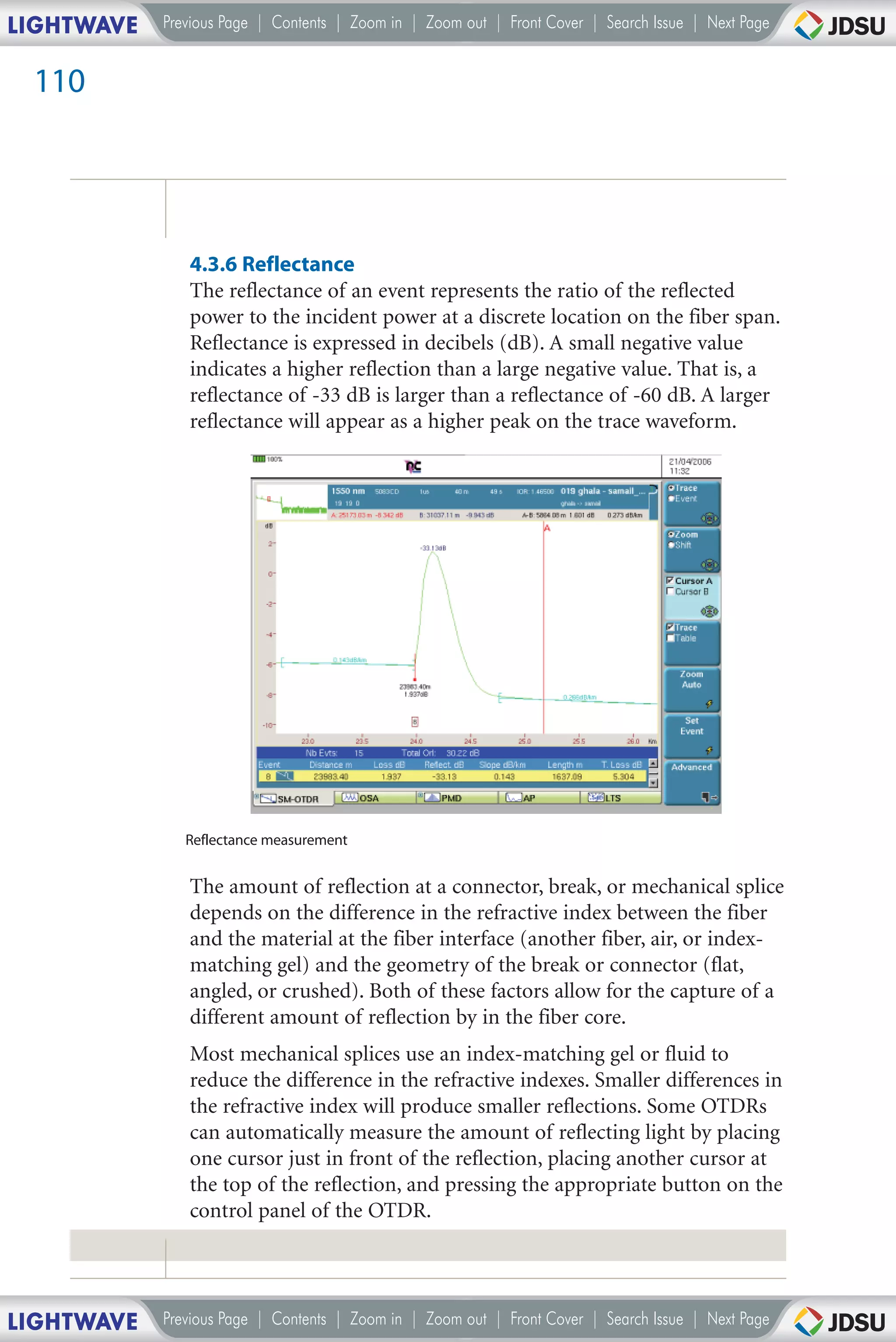
4.3.7 Optical Return Loss
High-performance OTDRs can automatically measure and report a
value for the total link optical return loss (ORL). A manual ORL
measurement capability is also provided in order to isolate the
portion of the link, which contributes the majority of the ORL.
4.3.7.1 Measuring ORL with an OTDR
The light received by an OTDR corresponds to the behavior of
the reflected power along the fiber link according to the injected
pulsewidth. The integral of this power allows for the calculation
of the total back reflection and for the determination of the
ORL value.
ORL=10 Log [(P0x∆t)/(∫Pr(z)dz)]
Where Po is the output power of the OTDR, ∆t is the OTDR
pulsewidth, and ∫Pr(z)dz is the total backreflected and backscattered
power over the distance (partial or total).
ORL measurement of a fiber link
LIGHTWAVE Previous Page | Contents | Zoom in | Zoom out | Front Cover | Search Issue | Next Page](https://image.slidesharecdn.com/jdsubook-130331001905-phpapp01/75/Jdsu-book-120-2048.jpg)


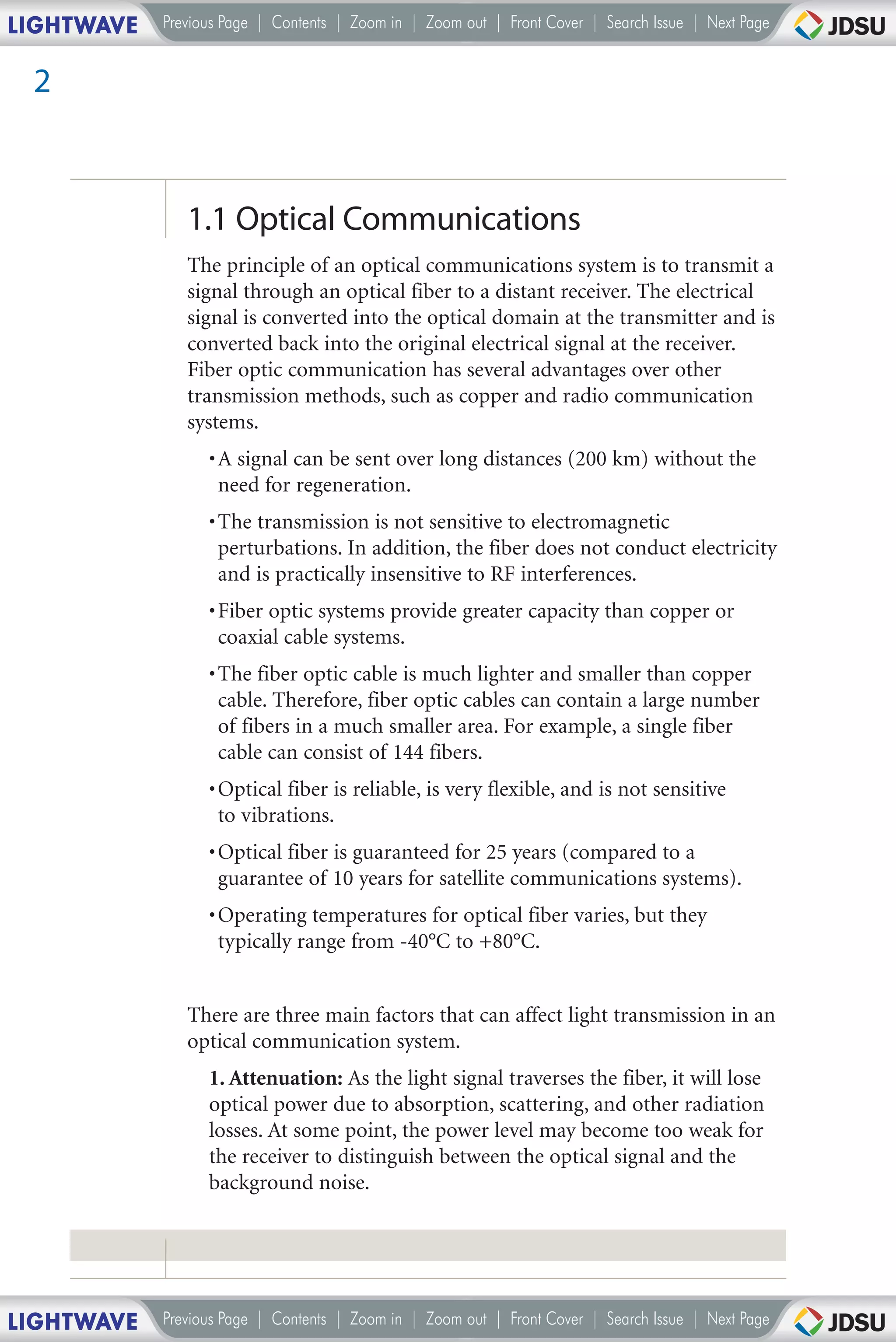
This document provides an overview and introduction to fiber optic testing and measurement. It discusses the basic principles of light transmission in optical fibers, including different fiber types, attenuation, dispersion, and other effects. It also describes common fiber optic test equipment used to measure insertion loss, return loss, and characterize fibers, such as light sources, power meters, loss test sets, optical time domain reflectometers (OTDRs), and monitoring systems. The document is intended to serve as a reference guide for fiber optic testing.


