Download as KEY, PPTX

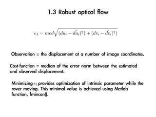
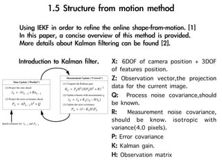
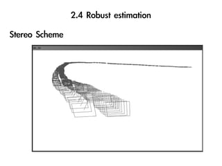
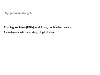
![Initial state estimate distribution
is done using batch algorithm[1]
to get mean and covariance.
This estimates initial 6D camera
positions corresponding to
several images in the sequence.
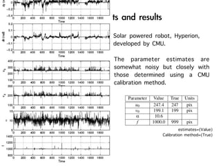
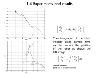
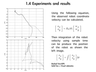
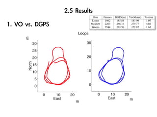
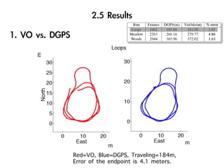
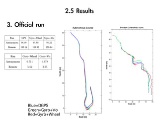
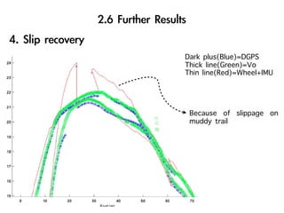
29.2m traveled and average
error=22.9cm and maximum
error=72.7cm.](https://image.slidesharecdn.com/visualodometrypresentationwithoutvideo-110508014736-phpapp01/85/Visual-odometry-presentation_without_video-34-320.jpg)
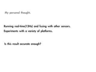
![2
E(u, v) = w(x, y)[I(x + u, y + v) − I(x, y)]
x,y
≈ [I(x, y) + uIx + vIy − I(x, y)]2
x,y
= u2 Ix + 2uvIx Iy + v 2 Iy
2 2
x,y
2
Ix Ix Iy u
= u v 2
Ix Iy Iy v
x,y
2
Ix Ix Iy u
= u v ( 2 )
Ix Iy Iy v
x,y
u 2
Ix Ix Iy
E(u, v) ∼
= u v M ,M = w(x, y) 2
v Ix Iy Iy
x,y](https://image.slidesharecdn.com/visualodometrypresentationwithoutvideo-110508014736-phpapp01/85/Visual-odometry-presentation_without_video-46-320.jpg)
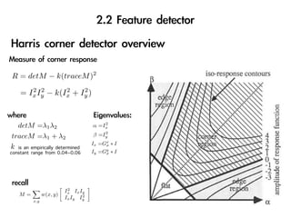
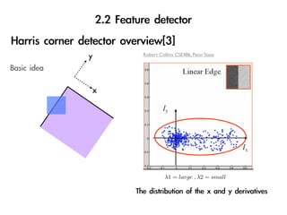
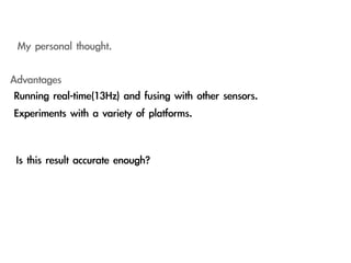
![R = detM − k(traceM )2
2 2 2 2
= Ix Iy − k(Ix + Iy )
2
detM =λ1 λ2 α =Ix
2
traceM =λ1 + λ2 β =Iy
Ix =Gx ∗ I
k is an empirically determined σ
constant range from 0.04~0.06 Iy =Gy ∗ I
σ
2
Ix Ix Iy
M= w(x, y) 2
Ix Iy Iy
x,y
Source from [3]](https://image.slidesharecdn.com/visualodometrypresentationwithoutvideo-110508014736-phpapp01/85/Visual-odometry-presentation_without_video-48-320.jpg)
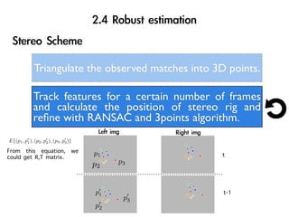
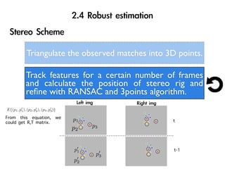


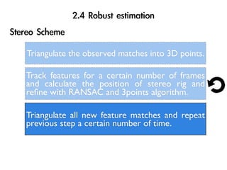
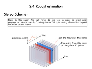


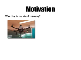
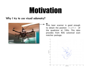
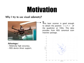
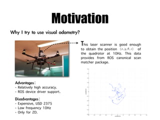
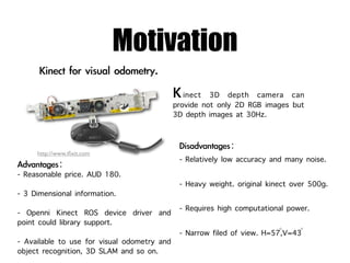
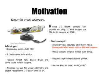
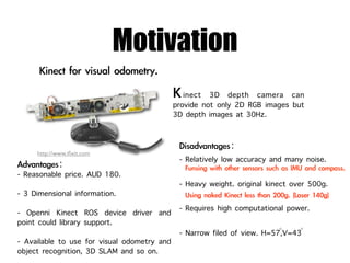
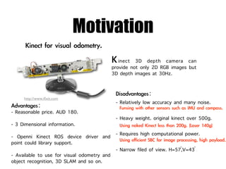
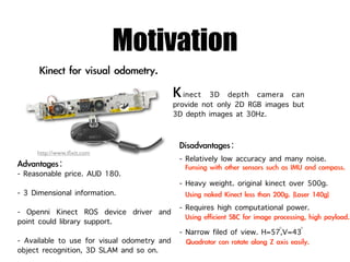
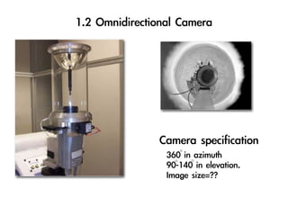
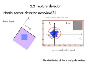
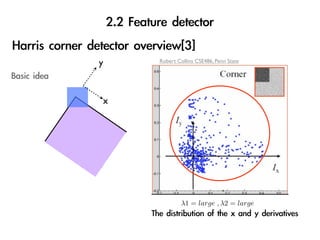
The document discusses visual odometry using laser and depth cameras, detailing their performance, accuracy, and applications. It highlights the Inect 3D depth camera's ability to capture 2D RGB and 3D depth images at 30Hz with reasonable pricing but notes its lower accuracy and high computational demands. It also covers techniques like RANSAC and triangulation for estimating positions and refining results in visual odometry.