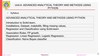
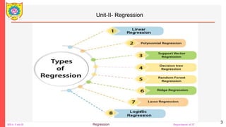
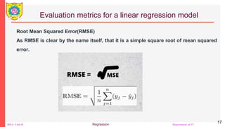
Course – Big Data Analytics (Professional
Elective-II)
Course code-IT314B
Unit-II- ADVANCED ANALYTICAL THEORY AND
METHODS USING PYTHON
Sanjivani Rural Education Society’s
Sanjivani College of Engineering, Kopargaon-423603
(An Autonomous Institute Affiliated to Savitribai Phule Pune University, Pune)
NAAC ‘A’ Grade Accredited, ISO 9001:2015 Certified
Department of Information Technology
(NBA Accredited)
Mr. Rajendra N Kankrale
Asst. Prof.
1
BDA- Unit-II Regression Department of IT
Unit-II- ADVANCED ANALYTICAL THEORY AND METHODS USING
PYTHON
• Syllabus
2
ADVANCED ANALYTICAL THEORY AND METHODS USING PYTHON
Introduction to Scikit-learn,
Installations, Dataset, matplotlib, filling missing values,
Regression and Classification using Scikit-learn
Association Rules: FP growth,
Regression: Linear Regression, Logistic Regression,
Classification: Naïve Bayes classifier
BDA- Unit-II Regression Department of IT
Unit-II- Regression
3
BDA- Unit-II Regression Department of IT
Unit-II- Regression
• Motivation
• Regression estimates the relationship between the target and
the independent variable.
• It is used to find the trends in data.
• It helps to predict real/continuous values.
• By performing the regression, we can confidently determine the
most important factor, the least important factor, and how each
factor is affecting the other factors.
4
BDA- Unit-II Regression Department of IT
Linear Regression
• Linear Regression is a supervised machine learning algorithm.
• It tries to find out the best linear relationship that describes the data you have.
• It assumes that there exists a linear relationship between a dependent variable and
independent variable(s).
• The value of the dependent variable of a linear regression model is a continuous
value i.e. real numbers.
5
BDA- Unit-II Regression Department of IT
Representing Linear Regression Model
• Linear regression model represents the linear relationship between a dependent
variable and independent variable(s) via a sloped straight line
• The sloped straight line representing the linear relationship that fits the given
data best is called as a regression line.
• It is also called as best fit line.
6
BDA- Unit-II Regression Department of IT
Types of Linear Regression-
1. Simple Linear Regression
2. Multiple Linear Regression
7
BDA- Unit-II Regression Department of IT
Simple Linear Regression
For simple linear regression, the form of the model is-
Y = β0 + β1X
8
Here,
Y is a dependent variable.
X is an independent variable.
β0 and β1 are the regression coefficients.
β0 is the intercept or the bias that fixes the offset to a
line.
β1 is the slope or weight that specifies the factor by
which X has an impact on Y.
BDA- Unit-II Regression Department of IT
Simple Linear Regression
There are following 3 cases possible-
Case-01: β1 < 0
It indicates that variable X has negative impact on Y.
If X increases, Y will decrease and vice-versa.
9
BDA- Unit-II Regression Department of IT
Simple Linear Regression
Case-02: β1 = 0
• It indicates that variable X has no impact on Y.
• If X changes, there will be no change in Y.
10
BDA- Unit-II Regression Department of IT
Simple Linear Regression
11
Case-03: β1 > 0
It indicates that variable X has positive impact on Y.
If X increases, Y will increase and vice-versa.
BDA- Unit-II Regression Department of IT
Multiple Linear Regression-
12
In multiple linear regression, the dependent variable depends on more
than one independent variables.
For multiple linear regression, the form of the model is-
Y = β0 + β1X1 + β2X2 + β3X3 + …… + βnXn
Here,
Y is a dependent variable.
X1, X2, …., Xn are independent variables.
β0, β1,…, βn are the regression coefficients.
βj (1<=j<=n) is the slope or weight that specifies the factor
by which Xj has an impact on Y.
BDA- Unit-II Regression Department of IT
Evaluation metrics for a linear regression model
Mean Squared Error (MSE)
The most common metric for regression tasks is MSE. It has a convex shape. It
is the average of the squared difference between the predicted and actual value.
Since it is differentiable and has a convex shape, it is easier to optimize.
MSE penalizes large errors.
13
BDA- Unit-II Regression Department of IT
Evaluation metrics for a linear regression model
14
BDA- Unit-II Regression Department of IT
Evaluation metrics for a linear regression model
Mean Absolute Error (MAE)
This is simply the average of the absolute difference between the target value
and the value predicted by the model. Not preferred in cases where outliers are
prominent.
MAE does not penalize large errors.
15
BDA- Unit-II Regression Department of IT
Evaluation metrics for a linear regression model
16
BDA- Unit-II Regression Department of IT
Evaluation metrics for a linear regression model
Root Mean Squared Error(RMSE)
As RMSE is clear by the name itself, that it is a simple square root of mean squared
error.
17
BDA- Unit-II Regression Department of IT
Evaluation metrics for a linear regression model
18
BDA- Unit-II Regression Department of IT
Evaluation metrics for a linear regression model
R-squared explains to what extent the variance of one variable explains
the variance of the second variable. In other words, it measures the
proportion of variance of the dependent variable explained by the
independent variable.
R squared is a popular metric for identifying model accuracy. It tells how
close are the data points to the fitted line generated by a regression
algorithm. A larger R squared value indicates a better fit. This helps us to
find the relationship between the independent variable towards the
dependent variable.
19
BDA- Unit-II Regression Department of IT
Evaluation metrics for a linear regression model
• SSE is the sum of the square of the
difference between the actual value
and the predicted value
• SST is the total sum of the square of
the difference between the actual
value and the mean of the actual
value.
• yi is the observed target value, ŷi is
the predicted value, and y-bar is the
mean value, m represents the total
number of observations.
20
BDA- Unit-II Regression Department of IT
Evaluation metrics for a linear regression model
21
BDA- Unit-II Regression Department of IT
Evaluation metrics for a linear regression model
22
• R² score ranges from 0 to 1. The closest to 1 the R², the better the
regression model is. If R² is equal to 0, the model is not performing better
than a random model. If R² is negative, the regression model is erroneous.
• A small MAE suggests the model is great at prediction, while a large MAE
suggests that your model may have trouble in certain areas. MAE of 0
means that your model is a perfect predictor of the outputs.
• If you have outliers in the dataset then it penalizes the outliers most and
the calculated MSE is bigger. So, in short, It is not Robust to outliers which
were an advantage in MAE.
BDA- Unit-II Regression Department of IT
Simple Linear Regression With scikit-learn
23
• You’ll start with the simplest case, which is simple linear regression. There
are five basic steps when you’re implementing linear regression:
1. Import the packages and classes that you need.
2. Provide data to work with, and eventually do appropriate transformations.
3. Create a regression model and fit it with existing data.
4. Check the results of model fitting to know whether the model is
satisfactory.
5. Apply the model for predictions.
BDA- Unit-II Regression Department of IT
Simple Linear Regression With scikit-learn
24
• Step 1: Import packages and classes
• The first step is to import the package numpy and the class
LinearRegression from sklearn.linear_model:
• >>> import numpy as np
• >>> from sklearn.linear_model import LinearRegression
BDA- Unit-II Regression Department of IT
Simple Linear Regression With scikit-learn
25
• Step 2: Provide data
• The second step is defining data to work with. The inputs (regressors, 𝑥)
and output (response, 𝑦) should be arrays or similar objects. This is the
simplest way of providing data for regression:
• >>> x = np.array([5, 15, 25, 35, 45, 55]).reshape((-1, 1))
• >>> y = np.array([5, 20, 14, 32, 22, 38])
• Now, you have two arrays: the input, x, and the output, y. You should call
.reshape() on x because this array must be two-dimensional, or more
precisely, it must have one column and as many rows as necessary. That’s
exactly what the argument (-1, 1) of .reshape() specifies.
BDA- Unit-II Regression Department of IT
Simple Linear Regression With scikit-learn
26
• This is how x and y look now:
• >>> x
• array([[ 5],
• [15],
• [25],
• [35],
• [45],
• [55]])
• >>> y
• array([ 5, 20, 14, 32, 22, 38])
• As you can see, x has two dimensions, and x.shape is (6, 1), while y has a
single dimension, and y.shape is (6,).
BDA- Unit-II Regression Department of IT
Simple Linear Regression With scikit-learn
27
• Step 3: Create a model and fit it
• The next step is to create a linear regression model and fit it using the
existing data.
• Create an instance of the class LinearRegression, which will represent the
regression model:
• >>> model = LinearRegression()
• This statement creates the variable model as an instance of
LinearRegression. You can provide several optional parameters to
LinearRegression:
BDA- Unit-II Regression Department of IT
Simple Linear Regression With scikit-learn
28
• This statement creates the variable model as an instance of
LinearRegression. You can provide several optional parameters to
LinearRegression:
• fit_intercept is a Boolean that, if True, decides to calculate the intercept 𝑏₀
or, if False, considers it equal to zero. It defaults to True.
• normalize is a Boolean that, if True, decides to normalize the input
variables. It defaults to False, in which case it doesn’t normalize the input
variables.
• copy_X is a Boolean that decides whether to copy (True) or overwrite the
input variables (False). It’s True by default.
• n_jobs is either an integer or None. It represents the number of jobs used
in parallel computation. It defaults to None, which usually means one job. -
1 means to use all available processors.
• Your model as defined above uses the default values of all parameters.
BDA- Unit-II Regression Department of IT
Simple Linear Regression With scikit-learn
29
• It’s time to start using the model. First, you need to call .fit() on model:
• >>> model.fit(x, y)
• LinearRegression()
• With .fit(), you calculate the optimal values of the weights 𝑏₀ and 𝑏₁, using
the existing input and output, x and y, as the arguments. In other words,
.fit() fits the model. It returns self, which is the variable model itself. That’s
why you can replace the last two statements with this one:
• >>> model = LinearRegression().fit(x, y)
• This statement does the same thing as the previous two. It’s just shorter.
BDA- Unit-II Regression Department of IT
Simple Linear Regression With scikit-learn
30
• Step 4: Get results
• Once you have your model fitted, you can get the results to check whether
the model works satisfactorily and to interpret it.
• You can obtain the coefficient of determination, 𝑅², with .score() called on
model:
• >>> r_sq = model.score(x, y)
• >>> print(f"coefficient of determination: {r_sq}")
• coefficient of determination: 0.7158756137479542
BDA- Unit-II Regression Department of IT
Simple Linear Regression With scikit-learn
31
• When you’re applying .score(), the arguments are also the predictor x and
response y, and the return value is 𝑅².
• The attributes of model are .intercept_, which represents the coefficient 𝑏₀,
and .coef_, which represents 𝑏₁:
• >>> print(f"intercept: {model.intercept_}")
• intercept: 5.633333333333329
• >>> print(f"slope: {model.coef_}")
• slope: [0.54]
• The code above illustrates how to get 𝑏₀ and 𝑏₁. You can notice that
.intercept_ is a scalar, while .coef_ is an array.

Unit2_Regression, ADVANCED ANALYTICAL THEORY AND METHODS USING PYTHON

  • 1.
    Course – BigData Analytics (Professional Elective-II) Course code-IT314B Unit-II- ADVANCED ANALYTICAL THEORY AND METHODS USING PYTHON Sanjivani Rural Education Society’s Sanjivani College of Engineering, Kopargaon-423603 (An Autonomous Institute Affiliated to Savitribai Phule Pune University, Pune) NAAC ‘A’ Grade Accredited, ISO 9001:2015 Certified Department of Information Technology (NBA Accredited) Mr. Rajendra N Kankrale Asst. Prof. 1
  • 2.
    BDA- Unit-II RegressionDepartment of IT Unit-II- ADVANCED ANALYTICAL THEORY AND METHODS USING PYTHON • Syllabus 2 ADVANCED ANALYTICAL THEORY AND METHODS USING PYTHON Introduction to Scikit-learn, Installations, Dataset, matplotlib, filling missing values, Regression and Classification using Scikit-learn Association Rules: FP growth, Regression: Linear Regression, Logistic Regression, Classification: Naïve Bayes classifier
  • 3.
    BDA- Unit-II RegressionDepartment of IT Unit-II- Regression 3
  • 4.
    BDA- Unit-II RegressionDepartment of IT Unit-II- Regression • Motivation • Regression estimates the relationship between the target and the independent variable. • It is used to find the trends in data. • It helps to predict real/continuous values. • By performing the regression, we can confidently determine the most important factor, the least important factor, and how each factor is affecting the other factors. 4
  • 5.
    BDA- Unit-II RegressionDepartment of IT Linear Regression • Linear Regression is a supervised machine learning algorithm. • It tries to find out the best linear relationship that describes the data you have. • It assumes that there exists a linear relationship between a dependent variable and independent variable(s). • The value of the dependent variable of a linear regression model is a continuous value i.e. real numbers. 5
  • 6.
    BDA- Unit-II RegressionDepartment of IT Representing Linear Regression Model • Linear regression model represents the linear relationship between a dependent variable and independent variable(s) via a sloped straight line • The sloped straight line representing the linear relationship that fits the given data best is called as a regression line. • It is also called as best fit line. 6
  • 7.
    BDA- Unit-II RegressionDepartment of IT Types of Linear Regression- 1. Simple Linear Regression 2. Multiple Linear Regression 7
  • 8.
    BDA- Unit-II RegressionDepartment of IT Simple Linear Regression For simple linear regression, the form of the model is- Y = β0 + β1X 8 Here, Y is a dependent variable. X is an independent variable. β0 and β1 are the regression coefficients. β0 is the intercept or the bias that fixes the offset to a line. β1 is the slope or weight that specifies the factor by which X has an impact on Y.
  • 9.
    BDA- Unit-II RegressionDepartment of IT Simple Linear Regression There are following 3 cases possible- Case-01: β1 < 0 It indicates that variable X has negative impact on Y. If X increases, Y will decrease and vice-versa. 9
  • 10.
    BDA- Unit-II RegressionDepartment of IT Simple Linear Regression Case-02: β1 = 0 • It indicates that variable X has no impact on Y. • If X changes, there will be no change in Y. 10
  • 11.
    BDA- Unit-II RegressionDepartment of IT Simple Linear Regression 11 Case-03: β1 > 0 It indicates that variable X has positive impact on Y. If X increases, Y will increase and vice-versa.
  • 12.
    BDA- Unit-II RegressionDepartment of IT Multiple Linear Regression- 12 In multiple linear regression, the dependent variable depends on more than one independent variables. For multiple linear regression, the form of the model is- Y = β0 + β1X1 + β2X2 + β3X3 + …… + βnXn Here, Y is a dependent variable. X1, X2, …., Xn are independent variables. β0, β1,…, βn are the regression coefficients. βj (1<=j<=n) is the slope or weight that specifies the factor by which Xj has an impact on Y.
  • 13.
    BDA- Unit-II RegressionDepartment of IT Evaluation metrics for a linear regression model Mean Squared Error (MSE) The most common metric for regression tasks is MSE. It has a convex shape. It is the average of the squared difference between the predicted and actual value. Since it is differentiable and has a convex shape, it is easier to optimize. MSE penalizes large errors. 13
  • 14.
    BDA- Unit-II RegressionDepartment of IT Evaluation metrics for a linear regression model 14
  • 15.
    BDA- Unit-II RegressionDepartment of IT Evaluation metrics for a linear regression model Mean Absolute Error (MAE) This is simply the average of the absolute difference between the target value and the value predicted by the model. Not preferred in cases where outliers are prominent. MAE does not penalize large errors. 15
  • 16.
    BDA- Unit-II RegressionDepartment of IT Evaluation metrics for a linear regression model 16
  • 17.
    BDA- Unit-II RegressionDepartment of IT Evaluation metrics for a linear regression model Root Mean Squared Error(RMSE) As RMSE is clear by the name itself, that it is a simple square root of mean squared error. 17
  • 18.
    BDA- Unit-II RegressionDepartment of IT Evaluation metrics for a linear regression model 18
  • 19.
    BDA- Unit-II RegressionDepartment of IT Evaluation metrics for a linear regression model R-squared explains to what extent the variance of one variable explains the variance of the second variable. In other words, it measures the proportion of variance of the dependent variable explained by the independent variable. R squared is a popular metric for identifying model accuracy. It tells how close are the data points to the fitted line generated by a regression algorithm. A larger R squared value indicates a better fit. This helps us to find the relationship between the independent variable towards the dependent variable. 19
  • 20.
    BDA- Unit-II RegressionDepartment of IT Evaluation metrics for a linear regression model • SSE is the sum of the square of the difference between the actual value and the predicted value • SST is the total sum of the square of the difference between the actual value and the mean of the actual value. • yi is the observed target value, ŷi is the predicted value, and y-bar is the mean value, m represents the total number of observations. 20
  • 21.
    BDA- Unit-II RegressionDepartment of IT Evaluation metrics for a linear regression model 21
  • 22.
    BDA- Unit-II RegressionDepartment of IT Evaluation metrics for a linear regression model 22 • R² score ranges from 0 to 1. The closest to 1 the R², the better the regression model is. If R² is equal to 0, the model is not performing better than a random model. If R² is negative, the regression model is erroneous. • A small MAE suggests the model is great at prediction, while a large MAE suggests that your model may have trouble in certain areas. MAE of 0 means that your model is a perfect predictor of the outputs. • If you have outliers in the dataset then it penalizes the outliers most and the calculated MSE is bigger. So, in short, It is not Robust to outliers which were an advantage in MAE.
  • 23.
    BDA- Unit-II RegressionDepartment of IT Simple Linear Regression With scikit-learn 23 • You’ll start with the simplest case, which is simple linear regression. There are five basic steps when you’re implementing linear regression: 1. Import the packages and classes that you need. 2. Provide data to work with, and eventually do appropriate transformations. 3. Create a regression model and fit it with existing data. 4. Check the results of model fitting to know whether the model is satisfactory. 5. Apply the model for predictions.
  • 24.
    BDA- Unit-II RegressionDepartment of IT Simple Linear Regression With scikit-learn 24 • Step 1: Import packages and classes • The first step is to import the package numpy and the class LinearRegression from sklearn.linear_model: • >>> import numpy as np • >>> from sklearn.linear_model import LinearRegression
  • 25.
    BDA- Unit-II RegressionDepartment of IT Simple Linear Regression With scikit-learn 25 • Step 2: Provide data • The second step is defining data to work with. The inputs (regressors, 𝑥) and output (response, 𝑦) should be arrays or similar objects. This is the simplest way of providing data for regression: • >>> x = np.array([5, 15, 25, 35, 45, 55]).reshape((-1, 1)) • >>> y = np.array([5, 20, 14, 32, 22, 38]) • Now, you have two arrays: the input, x, and the output, y. You should call .reshape() on x because this array must be two-dimensional, or more precisely, it must have one column and as many rows as necessary. That’s exactly what the argument (-1, 1) of .reshape() specifies.
  • 26.
    BDA- Unit-II RegressionDepartment of IT Simple Linear Regression With scikit-learn 26 • This is how x and y look now: • >>> x • array([[ 5], • [15], • [25], • [35], • [45], • [55]]) • >>> y • array([ 5, 20, 14, 32, 22, 38]) • As you can see, x has two dimensions, and x.shape is (6, 1), while y has a single dimension, and y.shape is (6,).
  • 27.
    BDA- Unit-II RegressionDepartment of IT Simple Linear Regression With scikit-learn 27 • Step 3: Create a model and fit it • The next step is to create a linear regression model and fit it using the existing data. • Create an instance of the class LinearRegression, which will represent the regression model: • >>> model = LinearRegression() • This statement creates the variable model as an instance of LinearRegression. You can provide several optional parameters to LinearRegression:
  • 28.
    BDA- Unit-II RegressionDepartment of IT Simple Linear Regression With scikit-learn 28 • This statement creates the variable model as an instance of LinearRegression. You can provide several optional parameters to LinearRegression: • fit_intercept is a Boolean that, if True, decides to calculate the intercept 𝑏₀ or, if False, considers it equal to zero. It defaults to True. • normalize is a Boolean that, if True, decides to normalize the input variables. It defaults to False, in which case it doesn’t normalize the input variables. • copy_X is a Boolean that decides whether to copy (True) or overwrite the input variables (False). It’s True by default. • n_jobs is either an integer or None. It represents the number of jobs used in parallel computation. It defaults to None, which usually means one job. - 1 means to use all available processors. • Your model as defined above uses the default values of all parameters.
  • 29.
    BDA- Unit-II RegressionDepartment of IT Simple Linear Regression With scikit-learn 29 • It’s time to start using the model. First, you need to call .fit() on model: • >>> model.fit(x, y) • LinearRegression() • With .fit(), you calculate the optimal values of the weights 𝑏₀ and 𝑏₁, using the existing input and output, x and y, as the arguments. In other words, .fit() fits the model. It returns self, which is the variable model itself. That’s why you can replace the last two statements with this one: • >>> model = LinearRegression().fit(x, y) • This statement does the same thing as the previous two. It’s just shorter.
  • 30.
    BDA- Unit-II RegressionDepartment of IT Simple Linear Regression With scikit-learn 30 • Step 4: Get results • Once you have your model fitted, you can get the results to check whether the model works satisfactorily and to interpret it. • You can obtain the coefficient of determination, 𝑅², with .score() called on model: • >>> r_sq = model.score(x, y) • >>> print(f"coefficient of determination: {r_sq}") • coefficient of determination: 0.7158756137479542
  • 31.
    BDA- Unit-II RegressionDepartment of IT Simple Linear Regression With scikit-learn 31 • When you’re applying .score(), the arguments are also the predictor x and response y, and the return value is 𝑅². • The attributes of model are .intercept_, which represents the coefficient 𝑏₀, and .coef_, which represents 𝑏₁: • >>> print(f"intercept: {model.intercept_}") • intercept: 5.633333333333329 • >>> print(f"slope: {model.coef_}") • slope: [0.54] • The code above illustrates how to get 𝑏₀ and 𝑏₁. You can notice that .intercept_ is a scalar, while .coef_ is an array.