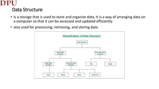
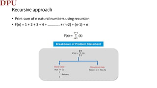
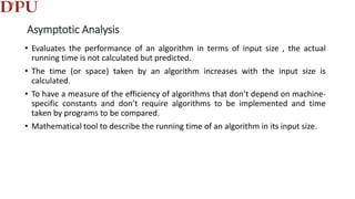
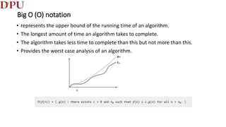
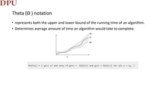
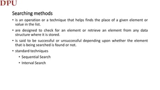
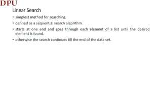
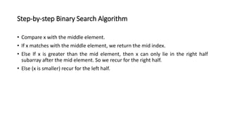
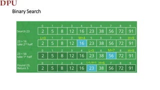
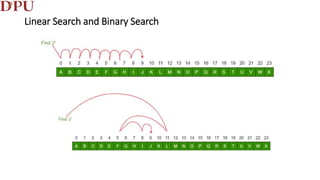
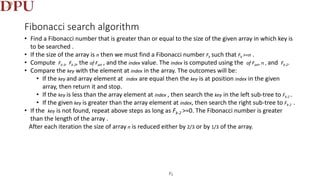
The document discusses various searching and sorting algorithms and data structures. It covers linear search and binary search algorithms. Linear search sequentially checks each element of a list to find a target value, while binary search works on a sorted list by dividing the search space in half at each step based on comparing the target to the middle element. The document also discusses asymptotic analysis techniques like Big O notation for analyzing algorithms' time and space complexity as input size increases.

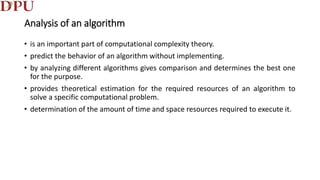

![Linear Search
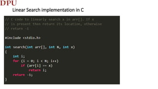
• Given an array arr[] of N elements, the task is to write a function to search a
given element x in arr[].
• Iterate from 0 to N-1 and compare the value of every index with x if they match
return index.](https://image.slidesharecdn.com/unitiisearchingandsortingalgorithms-221114044623-401f28d8/85/Unit-II_Searching-and-Sorting-Algorithms-ppt-31-320.jpg)
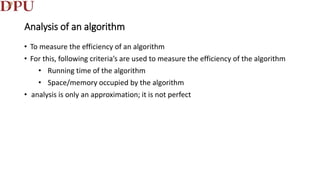
![Steps for Linear Search
• Start from the leftmost element of arr[] and one by one compare x with each
element of arr[].
• If x matches with an element, return the index.
• If x doesn’t match with any of the elements, return -1.](https://image.slidesharecdn.com/unitiisearchingandsortingalgorithms-221114044623-401f28d8/85/Unit-II_Searching-and-Sorting-Algorithms-ppt-32-320.jpg)
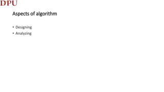
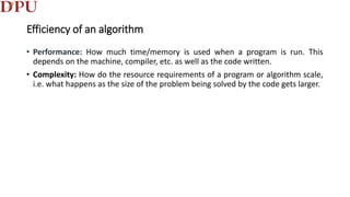
![Binary Search implementation
#include <stdio.h>
// A recursive binary search function. It returns location of x in given array arr[l..r] is present, otherwise -1
int binarySearch(int arr[], int l, int r, int x)
{
if (r >= l) {
int mid = l + (r - l) / 2;
// If the element is present at the middle itself
if (arr[mid] == x)
return mid;
// If element is smaller than mid, then it can only be present in left subarray
if (arr[mid] > x)
return binarySearch(arr, l, mid - 1, x);
// Else the element can only be present in right subarray
return binarySearch(arr, mid + 1, r, x);
}
// We reach here when element is not present in array
return -1;
}](https://image.slidesharecdn.com/unitiisearchingandsortingalgorithms-221114044623-401f28d8/85/Unit-II_Searching-and-Sorting-Algorithms-ppt-40-320.jpg)
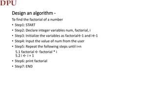
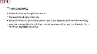
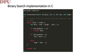
![Binary Search implementation
// A iterative binary search function. It returns location of x in given array arr[l..r] if present, otherwise -1
int binarySearch(int arr[], int l, int r, int x)
{
while (l <= r) {
int m = l + (r - l) / 2;
// Check if x is present at mid
if (arr[m] == x)
return m;
// If x greater, ignore left half
if (arr[m] < x)
l = m + 1;
// If x is smaller, ignore right half
else
r = m - 1;
}
// if we reach here, then element was not present
return -1;
}](https://image.slidesharecdn.com/unitiisearchingandsortingalgorithms-221114044623-401f28d8/85/Unit-II_Searching-and-Sorting-Algorithms-ppt-41-320.jpg)
![Example of Binary Search
int main(void)
{
int arr[] = { 2, 3, 4, 10, 40 };
int n = sizeof(arr) / sizeof(arr[0]);
int x = 10;
int result = binarySearch(arr, 0, n - 1, x);
(result == -1)
? printf("Element is not present in array")
: printf("Element is present at index %d", result);
return 0;
}](https://image.slidesharecdn.com/unitiisearchingandsortingalgorithms-221114044623-401f28d8/85/Unit-II_Searching-and-Sorting-Algorithms-ppt-42-320.jpg)


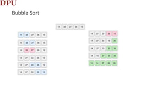
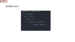
![Bubble Sort
// An optimized version of Bubble Sort
void bubbleSort(int arr[], int n)
{
int i, j;
bool swapped;
for (i = 0; i < n-1; i++)
{
swapped = false;
for (j = 0; j < n-i-1; j++)
{
if (arr[j] > arr[j+1])
{
swap(&arr[j], &arr[j+1]);
swapped = true;
}
}
// IF no two elements were swapped by inner loop, then
break
if (swapped == false)
break;
}
}
/* Function to print an array */
void printArray(int arr[], int size)
{
int i;
for (i=0; i < size; i++)
printf("%d ", arr[i]);
printf("n");
}
// Driver program to test above functions
int main()
{
int arr[] = {64, 34, 25, 12, 22, 11, 90};
int n = sizeof(arr)/sizeof(arr[0]);
bubbleSort(arr, n);
printf("Sorted array: n");
printArray(arr, n);
return 0;
}](https://image.slidesharecdn.com/unitiisearchingandsortingalgorithms-221114044623-401f28d8/85/Unit-II_Searching-and-Sorting-Algorithms-ppt-70-320.jpg)