Download to read offline

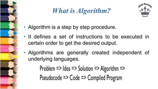

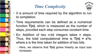
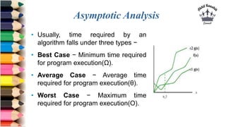
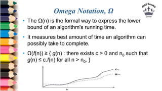
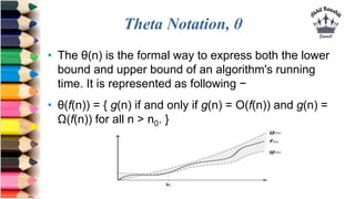
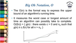
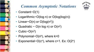
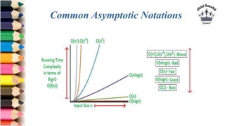
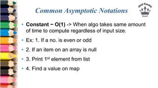
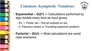
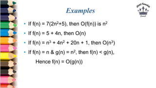
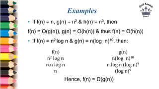
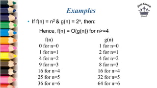


The document defines algorithms and describes their characteristics and design techniques. It states that an algorithm is a step-by-step procedure to solve a problem and get the desired output. It discusses algorithm development using pseudocode and flowcharts. Various algorithm design techniques like top-down, bottom-up, incremental, divide and conquer are explained. The document also covers algorithm analysis in terms of time and space complexity and asymptotic notations like Big-O, Omega and Theta to analyze best, average and worst case running times. Common time complexities like constant, linear, quadratic, and exponential are provided with examples.