Tv watching time project

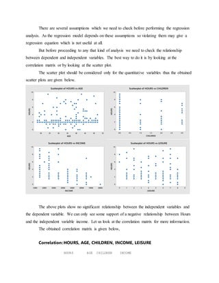
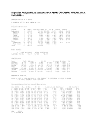
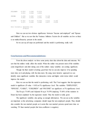
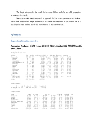
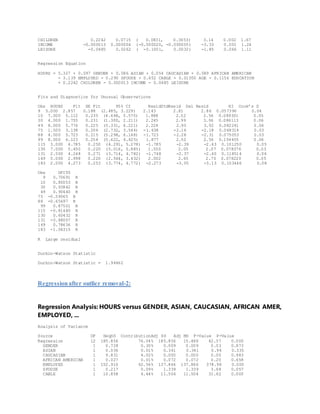
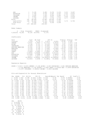
HEWLETT-PACKARD
[Type the document title]
[Type the document subtitle]
Surajit Basak
4/16/2015

Contents
Introduction .......................................................................................................................................1
Problem Statement..............................................................................................................................2
List of Technical Tasks .......................................................................................................................3
Data Description.................................................................................................................................3
Qualitative Variables:......................................................................................................................3
Quantitative Variables:....................................................................................................................4
Analysis:............................................................................................................................................4
Conclusions and Recommendations:..................................................................................................13
Appendix:.........................................................................................................................................14
Regression after outlier removal-1: ................................................................................................14
Regression after outlier removal-2: ................................................................................................15
Introduction
This regression class was very reallyinteresting; it not only taught us more about the
useful statistical techniques but also taught us the regression analysis.This is one of the most
important statistical tool used in professional world. Especially, the fact that we can predict the
future or another variable from already available data, which are collected from real world,
makesthe regression modeling so vital and useful. Therefore, we would like to build a regression
model using the collected data, so that we can use the learned materials in the real life data to
enhance our knowledge and practice the methods which will strengthen the learned knowledge.
The regression analysis can be used in many real life situations so getting the proper data
is not a problem. As the first step, we looked at few frequent activities in our daily life to get the
data. This is because, as these activities are done regularly (if not every day), we can collect data
from our daily life easily. The second step was,the result of this regression model should be
useful in our daily life. From these two approaches, we found TV watching as the topic.
Nowadays, most people watch TV and we can easily profile personal data for each person.
Moreover, TV watching time with general-personal data is significant to broadcasting companies,
TV manufacturers and advertising companies. If we get a significant regression model, these

companies can utilize the result to target the viewers based on the specific factors as they need.
For example, if people aged between 40-45 years old and within $30,000~$35,000 income range
has the highest TV watch time, the advertising companies should focus on the products which
these category wants.
We thought this will be a useful regression where we are learning by applying regression
model in the real world data.
Problem Statement
Though a high proportion of people watch television, but still some don’t and even the
viewing time and habit mostly depends on the personal choice like what kind of program they
like, their leisure time and so on. Therefore we set the target to capture the data from regular TV
watchers and who can possibly affect company’s profit. Statistically perceiving hours of the
people watching television will support companies to develop a strategy in advertisement.
In this report, we came up with various factors which can affect people’s TV watching
time. The factors such as their gender, race, employment, spouse presence, cable availability,
years of education, numbers of children, amount of income, and hours spent on leisure are
considered in this project. These factors are taken into account as independent variables in our
regression model in order to forecast the hours spend on TV watching. Our overall objective is to
give an idea about how the TV watching time can be differed by certain significant factors, and
later the companies can relate their advertisement to influence these factors to increase their
profit margin. As for example if we find out that Women tend to watch TV more than men then
the advertising companies can give advertises targeting the women more than men and that
definitely will increase their profit margin.

List of TechnicalTasks
Here our target is to find a proper regression model to predict the TV watching time
based on the other independent variables.
As regression model has many assumptions which should be fulfilled to consider the
model as valid. So we also need to run the assumptions check and need to make the correction if
necessary.
Here I will start with scatter diagram plot which will inform me whether there are any
linear relationship between the dependent and independent variables.
After looking at it I will start with regression analysis and see whether there are any
outliersin the data or not. If there are outliers found I will remove them till I have the data with
no significant outliers. This will take care of another assumption of the regression analysis.
Then I will select a subset model of the significant variables from the full model.
All the others assumptions will be check on this model to see whether the assumptions
are validated or not.
Data Description
Rather than collecting the data from online or from some other sources, our group
decided to physically collect the data, since we wanted to have our own data (which is more
accurate) rather than one collected by others. For accuracy, our group member went to several
different locations such as Georgia State, Atlantic Station, and Coca-Cola and selected random
people to collect the data, by selecting random people we tried to eliminate the data collection or
sampling bias. We used several different qualitative variables and quantitative variables for the
data collection. Below are the independent variables which we chose as these are really
important in affecting the TV watch time.
Qualitative Variables:

Gender: 1= Male and 0=Female (Qualitative variable with Nominal Scale)
Asian: 1= Asian and 0 = Non-Asian (Qualitative variable with Nominal Scale)
Caucasian: 1= Caucasian and 0 = Non-Caucasian (Qualitative variable with Nominal Scale)
African-American: 1= African-American and 0 = Non-African-American (Qualitative variable
with Nominal Scale)
Employment: 1= Viewer has a job, 0 = he/she does not (Qualitative variable with Nominal Scale)
Spouse: 1= Viewer is married, 0 = he/she is not (Qualitative variable with Nominal Scale)
Cable TV: 1= Viewer has cable connection, 0 = he/she does not (Qualitative variable with
Nominal Scale)
Education: Measurement of viewer's education level. (1 ~ High School Diploma, 2 ~ College, 3
~ Graduate school) (Qualitative variable with Ordinal Scale)
Quantitative Variables:
Age: Quantitative measurement of viewer's age (Quantitative variable with Ratio Scale)
Children: Quantitative measurement of viewer's number of children (Quantitative variable with
Ratio Scale)
Income: Quantitative measurement of viewer's income (Income range) (Quantitative variable
with Ratio Scale)
Leisure: Quantitative measurement of viewer's time spent on leisure (Hour spent on leisure
weekly) (Quantitative variable with Ratio Scale)
Our dependent variables is,
Hours: Hours spent on watching TV weekly (Quantitative variable with Ratio Scale)
Analysis:

There are several assumptions which we need to check before performing the regression
analysis. As the regression model depends on these assumptions so violating them may give a
regression equation which is not useful at all.
But before proceeding to any that kind of analysis we need to check the relationship
between dependent and independent variables. The best way to do it is by looking at the
correlation matrix or by looking at the scatter plot.
The scatter plot should be considered only for the quantitative variables thus the obtained
scatter plots are given below.
The above plots show no significant relationship between the independent variables and
the dependent variable. We can only see some support of a negative relationship between Hours
and the independent variable income. Let us look at the correlation matrix for more information.
The obtained correlation matrix is given below,
Correlation: HOURS, AGE, CHILDREN, INCOME, LEISURE
HOURS AGE CHILDREN INCOME
5550454035302520
10
8
6
4
2
0
AGE
HOURS
Scatterplot of HOURS vs AGE
3.02.52.01.51.00.50.0
10
8
6
4
2
0
CHILDREN
HOURS
Scatterplot of HOURS vs CHILDREN
8000070000600005000040000300002000010000
10
8
6
4
2
0
INCOME
HOURS
Scatterplot of HOURS vs INCOME
9876543210
10
8
6
4
2
0
LEISURE
HOURS
Scatterplot of HOURS vs LEISURE

AGE 0.037
0.601
CHILDREN 0.000 0.038
0.997 0.594
INCOME -0.375 0.011 0.124
0.000 0.877 0.079
LEISURE -0.123 -0.115 0.007 0.204
0.082 0.104 0.919 0.004
Cell Contents: Pearson correlation
P-Value
From the above result it is clear that only income has a significant correlation with the
hours. Though the result suggests that we should eliminate the variables which are not
significantly correlated with the dependent variable Hours but as we also have many qualitative
dummy variables so I am proceeding with taking these “insignificant” variables in my regression.
Before starting to analyze the data, we need to check the assumptions of regression analysis:
i) Linear relationship:
ii) Normality:
iii) No or little multicollinearity:
iv) Homoscedasticity:
v) No significant outliers in the model:
vi) No serial correlation in the model:
Now the 1st assumption is already validated through the scatter plots.
The all other assumptions can be checked before the regression analysis also but as we
may need to select a subset so I am keeping the assumptions check for the later part.
Considering all the independent variables the full regression model output is given below.
Regression Analysis: HOURS versus GENDER, ASIAN, CAUCASIAN, AFRICAN AMER,
EMPLOYED, ...
Analysis of Variance
Source DF SeqSS ContributionAdj SS Adj MS F-Value P-Value
Regression 12 342.100 54.39% 342.100 28.508 18.58 0.000
GENDER 1 0.126 0.02% 0.627 0.627 0.41 0.524

ASIAN 1 0.004 0.00% 0.458 0.458 0.30 0.585
CAUCASIAN 1 1.176 0.19% 2.751 2.751 1.79 0.182
AFRICAN AMERICAN 1 1.754 0.28% 0.255 0.255 0.17 0.684
EMPLOYED 1 268.434 42.68% 227.611 227.611 148.36 0.000
SPOUSE 1 0.220 0.03% 4.661 4.661 3.04 0.083
CABLE 1 27.197 4.32% 28.553 28.553 18.61 0.000
AGE 1 0.441 0.07% 1.435 1.435 0.94 0.335
EDUCATION 1 18.581 2.95% 5.963 5.963 3.89 0.050
CHILDREN 1 2.483 0.39% 4.527 4.527 2.95 0.088
INCOME 1 20.832 3.31% 18.628 18.628 12.14 0.001
LEISURE 1 0.852 0.14% 0.852 0.852 0.56 0.457
Error 187 286.900 45.61% 286.900 1.534
Lack-of-Fit 186 286.400 45.53% 286.400 1.540 3.08 0.431
Pure Error 1 0.500 0.08% 0.500 0.500
Total 199 629.000 100.00%
Model Summary
S R-sq R-sq(adj) PRESS R-sq(pred)
1.23864 54.39% 51.46% 329.350 47.64%
Coefficients
Term Coef SE Coef 95% CI T-Value P-Value VIF
Constant 5.944 0.502 ( 4.954, 6.934) 11.85 0.000
GENDER -0.116 0.181 ( -0.473, 0.242) -0.64 0.524 1.06
ASIAN 0.162 0.296 ( -0.422, 0.745) 0.55 0.585 1.86
CAUCASIAN 0.372 0.278 ( -0.176, 0.919) 1.34 0.182 2.09
AFRICAN AMERICAN 0.111 0.272 ( -0.426, 0.648) 0.41 0.684 2.16
EMPLOYED -3.050 0.250 ( -3.544, -2.556) -12.18 0.000 1.13
SPOUSE -0.397 0.228 ( -0.846, 0.052) -1.74 0.083 1.69
CABLE 0.793 0.184 ( 0.431, 1.156) 4.31 0.000 1.07
AGE 0.00898 0.00929 ( -0.00934, 0.02730) 0.97 0.335 1.12
EDUCATION -0.263 0.133 ( -0.526, 0.000) -1.97 0.050 1.27
CHILDREN 0.190 0.111 ( -0.028, 0.409) 1.72 0.088 1.66
INCOME -0.000021 0.000006 (-0.000032, -0.000009) -3.48 0.001 1.30
LEISURE -0.0294 0.0395 ( -0.1074, 0.0485) -0.75 0.457 1.11
Regression Equation
HOURS = 5.944 - 0.116 GENDER + 0.162 ASIAN + 0.372 CAUCASIAN + 0.111 AFRICAN AMERICAN
- 3.050 EMPLOYED - 0.397 SPOUSE + 0.793 CABLE + 0.00898 AGE - 0.263 EDUCATION
+ 0.190 CHILDREN - 0.000021 INCOME - 0.0294 LEISURE
Fits and Diagnostics for Unusual Observations
Obs HOURS Fit SE Fit 95% CI ResidStdResid Del Resid HI Cook’s D
3 5.000 2.021 0.318 (1.394, 2.648) 2.979 2.49 2.52 0.0659293 0.03
10 9.000 6.545 0.379 (5.797, 7.292) 2.455 2.08 2.10 0.0937056 0.03
11 9.500 2.964 0.291 (2.390, 3.538) 6.536 5.43 5.90 0.0552064 0.13
15 8.500 5.766 0.339 (5.096, 6.435) 2.734 2.30 2.32 0.0750477 0.03
62 9.500 6.274 0.333 (5.617, 6.930) 3.226 2.70 2.75 0.0720839 0.04
71 6.000 2.831 0.301 (2.237, 3.424) 3.169 2.64 2.68 0.0590371 0.03
83 7.000 2.951 0.331 (2.299, 3.603) 4.049 3.39 3.49 0.0712014 0.07
96 2.000 5.014 0.331 (4.361, 5.667) -3.014 -2.53 -2.56 0.0713602 0.04
99 3.000 5.445 0.310 (4.833, 6.057) -2.445 -2.04 -2.06 0.0627761 0.02
116 8.000 5.450 0.364 (4.732, 6.169) 2.550 2.15 2.18 0.0865024 0.03
120 5.500 2.874 0.297 (2.288, 3.461) 2.626 2.18 2.21 0.0576223 0.02
163 3.500 6.153 0.341 (5.481, 6.824) -2.653 -2.23 -2.25 0.0755750 0.03
188 3.000 5.362 0.391 (4.591, 6.134) -2.362 -2.01 -2.03 0.0996398 0.03
192 7.500 2.939 0.258 (2.431, 3.447) 4.561 3.76 3.91 0.0432661 0.05
Obs DFITS
3 0.67055 R
10 0.67568 R
11 1.42586 R
15 0.66147 R

62 0.76682 R
71 0.67157 R
83 0.96693 R
96 -0.71031 R
99 -0.53224 R
116 0.66936 R
120 0.54557 R
163 -0.64377 R
188 -0.67419 R
192 0.83049 R
R Large residual
Durbin-Watson Statistic
Durbin-Watson Statistic = 1.76295
From the above output we can clearly see that many variables are insignificant in the
model. Moreover though the overall regression model is significant but the R-square value is
54.39% implying only 54.39% of the variation is getting explained by the regression model.
As many variables are insignificant so we should select some model with removing all
these insignificant variables. But as there are many outliers in the data (which can cause some
variable to be insignificant) so I am removing these outliers at first.
As we know for normal distribution 95%, 99.73% of the values fall within 2 and 3
standard deviation of the mean respectively. So lets remove all data points having standardized
residual value more than +2 or less than -2. After deleting them and running the regression
model the obtained output is given in Appendix: Regression after outlier removal-1.
We can still see some outliers falling in the outside of 2 standard deviation interval. By
keep deleting those data points and rerunning the model we reached at the point where no
standardized residuals have value outside 3 standard deviation interval.
As there is a 5% chance that the standardized residual will be outside 2 standard
deviation interval so I am keeping this dataset and running the stepwise selection method with
alpha to enter as 0.05 and alpha to remove as 0.15.
The obtained model is given below. All the in between regression output is given in the
appendix with proper numberings.

EMPLOYED, ...
Stepwise Selection of Terms
α to enter = 0.05, α to remove = 0.15
Regression 6 184.481 75.48% 184.481 30.747 85.66 0.000
EMPLOYED 1 162.047 66.30% 142.103 142.103 395.88 0.000
SPOUSE 1 0.075 0.03% 1.551 1.551 4.32 0.039
CABLE 1 11.339 4.64% 12.425 12.425 34.61 0.000
CHILDREN 1 2.968 1.21% 4.224 4.224 11.77 0.001
INCOME 1 6.257 2.56% 4.870 4.870 13.57 0.000
LEISURE 1 1.795 0.73% 1.795 1.795 5.00 0.027
Error 167 59.945 24.52% 59.945 0.359
Lack-of-Fit 166 59.445 24.32% 59.445 0.358 0.72 0.761
Pure Error 1 0.500 0.20% 0.500 0.500
Total 173 244.425 100.00%
Model Summary
0.599125 75.48% 74.59% 66.7525 72.69%
Coefficients
Constant 5.572 0.196 ( 5.186, 5.959) 28.47 0.000
EMPLOYED -3.193 0.160 ( -3.509, -2.876) -19.90 0.000 1.10
SPOUSE -0.242 0.116 ( -0.472, -0.012) -2.08 0.039 1.64
CABLE 0.5500 0.0935 ( 0.3654, 0.7345) 5.88 0.000 1.03
CHILDREN 0.1946 0.0567 ( 0.0826, 0.3066) 3.43 0.001 1.67
INCOME -0.000011 0.000003 (-0.000017, -0.000005) -3.68 0.000 1.13
LEISURE -0.0450 0.0201 ( -0.0847, -0.0053) -2.24 0.027 1.04
Regression Equation
HOURS = 5.572 - 3.193 EMPLOYED - 0.242 SPOUSE + 0.5500 CABLE + 0.1946 CHILDREN
- 0.000011 INCOME - 0.0450 LEISURE
1 0.500 1.715 0.088 (1.541, 1.888) -1.215 -2.05 -2.07 0.021474 0.01
8 0.500 2.082 0.090 (1.904, 2.260) -1.582 -2.67 -2.72 0.022635 0.02
16 0.000 1.247 0.145 (0.960, 1.534) -1.247 -2.15 -2.17 0.058811 0.04
21 7.000 5.823 0.173 (5.481, 6.165) 1.177 2.05 2.07 0.083517 0.05
29 0.000 1.466 0.128 (1.214, 1.718) -1.466 -2.50 -2.55 0.045412 0.04
47 0.000 1.379 0.118 (1.147, 1.612) -1.379 -2.35 -2.38 0.038685 0.03
49 7.000 5.835 0.195 (5.449, 6.220) 1.165 2.06 2.08 0.106367 0.07
58 7.500 5.928 0.169 (5.594, 6.262) 1.572 2.74 2.79 0.079613 0.09
73 4.000 5.321 0.171 (4.983, 5.658) -1.321 -2.30 -2.33 0.081243 0.07
80 3.500 4.817 0.168 (4.486, 5.149) -1.317 -2.29 -2.32 0.078552 0.06
87 4.500 3.109 0.201 (2.712, 3.506) 1.391 2.46 2.50 0.112469 0.11
95 7.000 5.781 0.168 (5.449, 6.112) 1.219 2.12 2.14 0.078559 0.05
106 0.000 1.409 0.113 (1.185, 1.633) -1.409 -2.39 -2.43 0.035807 0.03
110 4.000 5.214 0.186 (4.847, 5.581) -1.214 -2.13 -2.16 0.096315 0.07
115 3.500 2.157 0.092 (1.975, 2.338) 1.343 2.27 2.30 0.023601 0.02
Obs DFITS
1 -0.306549 R

8 -0.414255 R
16 -0.542294 R
21 0.625467 R
29 -0.555239 R
47 -0.477636 R
49 0.716874 R
58 0.820652 R
73 -0.692789 R
80 -0.677400 R
87 0.891054 R
95 0.625761 R
106 -0.468253 R
110 -0.703592 R
115 0.357270 R
R Large residual
Here we can see that quite few variables came to be significant. Though some residuals
are outside 2 standard deviation interval but none are outside 3 standard deviation interval. As
there are 174 data points here so 9 of the residuals are expected to be outside the 2 standard
deviation by normality rule and we can see that the number of residuals which is outside the 2
standard deviation interval is 15 which is close.
By applying the above method we also took care of the 5th assumption which is “No
significant outliers in the model”.
Now lets check the other assumptions.
The normality check can be done using the Normal probability plot of the residuals which
is given below.

From the above plot no significant deviation is found and thus normality assumption is
validated.
Similarly the Homoscedasticity assumption can be tested using the Residual vs Fit plot
which is given below.

The plot suggests a little deviation from the randomness however all values are within the
3 standard deviation. So ignoring this little deviation we can say that the Homoscedasticity
assumption is validated.
The Durbin-Watson Statistic = 1.76295 implying no significant serial correlation thus
another assumption is validated.
The last assumption is the multicollinearity which can be checked using the Variance
Inflation Factors (VIFs) we can see all VIFs have low values implying no multicollinearity in the
mode. Letscheck the correlation matrix to be sure.
The correlation matrix is given below,
As many variables are qualitative here so using the proper correlation method the
obtained output is given below,
Spearman Rho: EMPLOYED, SPOUSE, CABLE, CHILDREN, INCOME, LEISURE
EMPLOYED SPOUSE CABLE CHILDREN INCOME
SPOUSE -0.016
0.838
CABLE 0.112 0.091
0.139 0.231

CHILDREN -0.050 0.694 -0.016
0.511 0.000 0.833
INCOME 0.245 0.062 0.057 0.128
0.001 0.420 0.452 0.092
LEISURE -0.067 -0.030 -0.036 0.012 0.162
0.377 0.695 0.640 0.877 0.033
Cell Contents: Spearman rho
P-Value
Here we can see two obvious significance between “Income and employed” and “Spouse
and Children”. But as we saw that the Variance Inflation Factors for all variables are low so there
is no multicollinearity present in the model.
So we can say all steps are performed and the model is performing really well.
Conclusions and Recommendations:
From the above analysis we have some pretty clear idea about the data and outcome. We
saw that the outliers really affect the model. When the outlier was present most of the variables
came insignificant and after taking care of the outliers many variables are coming significant.
Though the final model is looking good here but we can also improve it by spending
more time on it and playing with the data more. By using more iterative approach we can
identify more significant variables like interaction terms and higher order terms which would
improve the model.
Here we can see that the model is performing well. The F test suggests that the regression
model is significant (P-value < 0.05) at 5% significance level. The variables “EMPLOYED”,
“SPOUSE”, “CABLE”, “CHILDREN” and “INCOME” are significant at 5% significance level.
The R-sq is 75.48% and Adjusted R-sq is 74.59% implying 75.48% of the variation in
Hours has been explained by the regression model. Thus the model is really good.
The significant variables also giving us enough information. We can see as the variables
are important so the advertising companies should target the non-employed people. They should
also consider the non married people as it seems like non married persons spend more time on
watching TV than married people (the beta coefficient is negative).

The should also consider the people having more children and who has cable connection
to optimize their profit.
But the regression model suggested to approach the less income persons as well as less
leisure time people which might be a mistake. We should run more tests to see whether this is a
fact or just a small mistake due to the characteristic of the collected data.
Appendix:
Regressionafter outlier removal-1:
EMPLOYED, ...
Regression 12 258.689 70.75% 258.689 21.557 34.87 0.000
GENDER 1 3.991 1.09% 0.413 0.413 0.67 0.415
ASIAN 1 0.731 0.20% 0.121 0.121 0.20 0.659
CAUCASIAN 1 11.922 3.26% 0.055 0.055 0.09 0.766
EMPLOYED 1 199.412 54.54% 190.482 190.482 308.07 0.000
SPOUSE 1 0.462 0.13% 2.276 2.276 3.68 0.057
CABLE 1 18.445 5.04% 17.970 17.970 29.06 0.000
AGE 1 1.704 0.47% 1.843 1.843 2.98 0.086
EDUCATION 1 5.017 1.37% 1.086 1.086 1.76 0.187
CHILDREN 1 4.703 1.29% 6.084 6.084 9.84 0.002
INCOME 1 8.544 2.34% 6.837 6.837 11.06 0.001
LEISURE 1 2.116 0.58% 2.116 2.116 3.42 0.066
Error 173 106.967 29.25% 106.967 0.618
Lack-of-Fit 172 106.467 29.12% 106.467 0.619 1.24 0.630
Pure Error 1 0.500 0.14% 0.500 0.500
Total 185 365.656 100.00%
Model Summary
0.786324 70.75% 68.72% 126.045 65.53%
Coefficients
Constant 5.327 0.341 ( 4.654, 6.000) 15.62 0.000
GENDER 0.097 0.119 ( -0.138, 0.332) 0.82 0.415 1.05
ASIAN 0.086 0.195 ( -0.298, 0.470) 0.44 0.659 1.78
CAUCASIAN 0.054 0.182 ( -0.305, 0.414) 0.30 0.766 2.06
AFRICAN AMERICAN 0.089 0.177 ( -0.260, 0.438) 0.50 0.614 2.12
EMPLOYED -3.139 0.179 ( -3.492, -2.786) -17.55 0.000 1.12
SPOUSE -0.290 0.151 ( -0.588, 0.008) -1.92 0.057 1.72
CABLE 0.652 0.121 ( 0.413, 0.890) 5.39 0.000 1.07
AGE 0.01050 0.00608 ( -0.00150, 0.02251) 1.73 0.086 1.11
EDUCATION -0.1156 0.0872 ( -0.2878, 0.0565) -1.33 0.187 1.26

CHILDREN 0.2242 0.0715 ( 0.0831, 0.3653) 3.14 0.002 1.67
INCOME -0.000013 0.000004 (-0.000020, -0.000005) -3.33 0.001 1.24
LEISURE -0.0485 0.0262 ( -0.1001, 0.0032) -1.85 0.066 1.11
Regression Equation
HOURS = 5.327 + 0.097 GENDER + 0.086 ASIAN + 0.054 CAUCASIAN + 0.089 AFRICAN AMERICAN
9 5.000 2.857 0.188 (2.485, 3.229) 2.143 2.81 2.86 0.057396 0.04
10 7.000 5.112 0.235 (4.648, 5.575) 1.888 2.52 2.56 0.089301 0.05
30 4.000 1.755 0.231 (1.300, 2.211) 2.245 2.99 3.06 0.086113 0.06
49 8.000 5.776 0.225 (5.331, 6.221) 2.224 2.95 3.02 0.082241 0.06
75 1.500 3.138 0.206 (2.732, 3.544) -1.638 -2.16 -2.18 0.068314 0.03
88 4.000 5.723 0.215 (5.298, 6.148) -1.723 -2.28 -2.31 0.075053 0.03
99 8.000 6.123 0.254 (5.622, 6.625) 1.877 2.52 2.56 0.104455 0.06
115 3.000 4.785 0.250 (4.291, 5.278) -1.785 -2.39 -2.43 0.101250 0.05
130 7.000 5.450 0.220 (5.016, 5.885) 1.550 2.05 2.07 0.078376 0.03
131 2.500 4.248 0.271 (3.714, 4.782) -1.748 -2.37 -2.40 0.118514 0.06
149 5.000 2.998 0.220 (2.564, 3.432) 2.002 2.65 2.70 0.078220 0.05
183 2.000 4.273 0.253 (3.774, 4.772) -2.273 -3.05 -3.13 0.103446 0.08
Obs DFITS
9 0.70691 R
10 0.80053 R
30 0.93842 R
49 0.90440 R
75 -0.59065 R
88 -0.65697 R
99 0.87501 R
115 -0.81480 R
130 0.60432 R
131 -0.88007 R
149 0.78636 R
183 -1.06315 R
R Large residual
Regressionafter outlier removal-2:
EMPLOYED, ...
Regression 12 185.856 76.04% 185.856 15.488 42.57 0.000
GENDER 1 0.728 0.30% 0.009 0.009 0.03 0.873
ASIAN 1 0.036 0.01% 0.341 0.341 0.94 0.335
CAUCASIAN 1 9.831 4.02% 0.000 0.000 0.00 0.983
EMPLOYED 1 152.910 62.56% 137.866 137.866 378.98 0.000
SPOUSE 1 0.217 0.09% 1.339 1.339 3.68 0.057
CABLE 1 10.858 4.44% 11.504 11.504 31.62 0.000

AGE 1 0.195 0.08% 0.193 0.193 0.53 0.467
EDUCATION 1 1.706 0.70% 0.187 0.187 0.52 0.474
CHILDREN 1 3.180 1.30% 4.262 4.262 11.72 0.001
INCOME 1 4.431 1.81% 3.477 3.477 9.56 0.0 02
LEISURE 1 1.736 0.71% 1.736 1.736 4.77 0.030
Error 161 58.569 23.96% 58.569 0.364
Lack-of-Fit 160 58.069 23.76% 58.069 0.363 0.73 0.758
Pure Error 1 0.500 0.20% 0.500 0.500
Total 173 244.425 100.00%
Model Summary
0.603145 76.04% 74.25% 69.9706 71.37%
Coefficients
Constant 5.518 0.276 ( 4.973, 6.063) 19.99 0.000
GENDER 0.0151 0.0943 ( -0.1712, 0.2014) 0.16 0.873 1.05
ASIAN 0.146 0.151 ( -0.152, 0.444) 0.97 0.335 1.75
CAUCASIAN -0.003 0.143 ( -0.285, 0.279) -0.02 0.983 2.00
AFRICAN AMERICAN -0.061 0.138 ( -0.334, 0.211) -0.44 0.658 2.01
EMPLOYED -3.232 0.166 ( -3.560, -2.904) -19.47 0.000 1.16
SPOUSE -0.230 0.120 ( -0.467, 0.007) -1.92 0.057 1.72
CABLE 0.5409 0.0962 ( 0.3509, 0.7308) 5.62 0.000 1.08
AGE 0.00354 0.00486 ( -0.00605, 0.01313) 0.73 0.467 1.13
EDUCATION -0.0494 0.0688 ( -0.1853, 0.0865) -0.72 0.474 1.29
CHILDREN 0.1977 0.0577 ( 0.0836, 0.3117) 3.42 0.001 1.70
INCOME -0.000010 0.000003 (-0.000016, -0.000004) -3.09 0.002 1.29
LEISURE -0.0453 0.0208 ( -0.0863, -0.0044) -2.18 0.030 1.10
Regression Equation
HOURS = 5.518 + 0.0151 GENDER + 0.146 ASIAN - 0.003 CAUCASIAN - 0.061 AFRICAN AMERICAN
1 0.500 1.914 0.148 (1.622, 2.205) -1.414 -2.42 -2.45 0.059821 0.03
8 0.500 1.965 0.133 (1.703, 2.226) -1.465 -2.49 -2.53 0.048293 0.02
16 0.000 1.319 0.193 (0.938, 1.701) -1.319 -2.31 -2.34 0.102496 0.05
21 7.000 5.720 0.205 (5.315, 6.124) 1.280 2.26 2.29 0.115574 0.05
23 3.500 2.303 0.127 (2.053, 2.554) 1.197 2.03 2.05 0.044229 0.01
29 0.000 1.392 0.159 (1.079, 1.706) -1.392 -2.39 -2.43 0.069151 0.03
33 6.000 4.838 0.193 (4.457, 5.219) 1.162 2.03 2.05 0.102488 0.04
47 0.000 1.365 0.159 (1.052, 1.679) -1.365 -2.35 -2.38 0.069404 0.03
58 7.500 5.869 0.182 (5.509, 6.229) 1.631 2.84 2.90 0.091226 0.06
73 4.000 5.479 0.232 (5.021, 5.936) -1.479 -2.66 -2.71 0.147459 0.09
80 3.500 4.719 0.194 (4.336, 5.103) -1.219 -2.14 -2.16 0.103423 0.04
87 4.500 3.152 0.223 (2.711, 3.593) 1.348 2.41 2.44 0.137104 0.07
94 1.500 2.789 0.193 (2.409, 3.170) -1.289 -2.26 -2.29 0.101942 0.04
106 0.000 1.337 0.149 (1.042, 1.631) -1.337 -2.29 -2.32 0.061106 0.03
115 3.500 2.116 0.135 (1.848, 2.383) 1.384 2.36 2.39 0.050391 0.02
Obs DFITS
1 -0.61923 R
8 -0.57008 R
16 -0.79113 R
21 0.82669 R
23 0.44095 R
29 -0.66204 R
33 0.69405 R
47 -0.65010 R
58 0.91922 R

73 -1.12589 R
80 -0.73343 R
87 0.97371 R
94 -0.76986 R
106 -0.59129 R
115 0.55046 R
R Large residual

Tv watching time project

More Related Content

What's hot

Viewers also liked

Similar to Tv watching time project

Recently uploaded

Tv watching time project