This document provides information about the Computational Chemistry 126 course offered at UC Santa Barbara in Fall 2011, including the instructor's contact information, course objectives, required readings and assignments. The course focuses on learning principles of computational chemistry and molecular modeling techniques. Students will learn algorithms for geometry optimization, transition state location, and prediction of molecular properties using software for quantum chemical calculations and molecular simulations.

1. Chem 126
Computational
Chemistry
Fall 2011
Lecturer:
Dr. Kalju Kahn
Office: PSB-N 2623, Phone: 893-6157
E-mail: kalju@chem.ucsb.edu, Website: http://www.chem.ucsb.edu/~kalju
Mission statement
The course focuses on learning the principles of computational chemistry and computer-based
molecular design. Both molecular mechanical and quantum mechanical models are covered.
Students will learn a variety of commonly used techniques, such as geometry optimization,
location of transition states, conformational analysis, and prediction of molecular and
spectroscopic properties. Students will learn basics of implementing key algorithms, such as
Newton-Rhapson minimization, and normal mode analysis of vibrational motions. Students also
will become familiar with different software packages, including MOLDEN for general model
building, Gaussian, Firefly, and NWChem for quantum chemical calculations, and BOSS for
liquid simulations. Students who complete the course are expected to be able to ask questions
that can be solved with modern computational approaches and choose right computational tools
to assist in their current or future research.
CourseMaterials
Syllabus General informationaboutthe course PDF
Last Years Computational Chemistry126by Dr. Kahn: 2008 Link
Last Years Computational Chemistry126by Dr. Kirtman:2007 Link
Textbook Suggested:IntoductiontoComputationalChemistry:TheoriesandModels Amazon
Textbook Alternative:Essentialsof ComputationalChemistry:TheoriesandModels Amazon
Upload SubmityourassignmentsasMS Word or PDF files Link

2. Exam MidtermPreparationGuide PDF
Exam Final PreparationGuide PDF
Literature
Literature Requiredoroptional readinginPDF Acrobat
Required "Mathematical Methods"byFrankJensen PDF
Required "OptimizationTechniques"byFrankJensen PDF
Required "Force FieldMethods"byFrankJensen PDF
Required "Biomolecularsimulationandmodelling:Status..."byvanderKamp et al PDF
Required "Potential energyfunctionsforatomic-level simulationsof waterandorganicand
biomolecularsystems"byJorgensenandTirado-Rives
PDF
Required IntroQuantumMechanics: MO Theory PDF
Optional BasisSetsfor AbInitioMO Calculations... PDF
Required DFT: Performance andProblems PDF
Optional "Performance of B3LYP DensityFunctionalMethods..."byTirado-RivesandJorgensen PDF
Optional Explanationof ThermochemistryatNIST Link
Assignments
The assignments are posted one week before the due date. Answers shall be submitted
electronically no later than the midnight of the due date.
Assignments SubmitYour Work Link
1 Minimization:Tutorial andAssignments Link
2 Molecules:Building,Minimization,andConformational Analysis Link

3. 3.a Monte Carlo Simulations Link
3.b IntroductiontoQM andSemiempirical Methods Link
4 IntroductiontoAnInitioMethods Link
5 MolecularVibrations Link
5 ReactionThermodynamics andKinetics:TransitionStates Link
6 NotRequired:ElectronicSpectraandSolventEffects Link
6 NotRequired:QM/MMModelingof Reactions:Free EnergyPerturbation Link
Answer Keys
The answer keys are posted one week after the due date.
ComputationalChemistry Links
Computational Chemistry List
Course materialsby Dr.KaljuKahn,Departmentof ChemistryandBiochemistry ,UC Santa Barbara. 2011

4. Tutorial Example for Methylamine
Running an NBO Calculation
This page provides an introductory quick-start tutorial on running an NBO calculation and
interpreting the output. The example chosen is that of methylamine (CH3NH2) in Pople-Gordon
idealized geometry, treated at the ab initio RHF/3-21G level. This simple split-valence basis set
consists of 28 AOs (nine each on C and N, two on each H), extended by 13 AOs beyond the
minimal basis level.
Input files to perform this calculation are
given here for Gaussian and GAMESS.
The pop=nbo option of the Gaussian
program requests default NBO analysis.
NBO analysis is requested in the
GAMESS calculation by simply
including the line
$NBO $END
in the GAMESS input file. This "empty"
NBO keylist specifies that NBO analysis
should be carried out at the default level.
The default NBO output produced by this example is shown below, just as it appears in your
output file. The start of the NBO section is marked by a standard header, citation, job title, and
storage info:
*********************************** NBO 5.0
***********************************
N A T U R A L A T O M I C O R B I T A L A N D
N A T U R A L B O N D O R B I T A L A N A L Y S I S
*****************************************************************************
**
(c) Copyright 1996-2001 Board of Regents of the University of Wisconsin
System
on behalf of the Theoretical Chemistry Institute. All Rights Reserved.
Cite this program as:
NBO 5.0. E. D. Glendening, J. K. Badenhoop, A. E. Reed,
J. E. Carpenter, J. A. Bohmann, C. M. Morales, and F. Weinhold
(Theoretical Chemistry Institute, University of Wisconsin,
Madison, WI, 2001)

5. Job title: Methylamine...RHF/3-21G//Pople-Gordon standard geometry
Storage needed: 2562 in NPA, 3278 in NBO ( 2000000
available)
Note that all NBO output is formatted to a maximum 80-character width for convenient display.
The NBO heading echoes any requested keywords (none for the present default case).
Natural Population Analysis
The next four NBO output segments summarize the results of natural population analysis (NPA).
The first segment is the main NAO table, as shown below:
NATURAL POPULATIONS: Natural atomic orbital occupancies
NAO Atom # lang Type(AO) Occupancy Energy
---------------------------------------------------------
1 C 1 s Cor( 1s) 1.99900 -11.04184
2 C 1 s Val( 2s) 1.09038 -0.28186
3 C 1 s Ryd( 3s) 0.00068 1.95506
4 C 1 px Val( 2p) 0.89085 -0.01645
5 C 1 px Ryd( 3p) 0.00137 0.93125
6 C 1 py Val( 2p) 1.21211 -0.07191
7 C 1 py Ryd( 3p) 0.00068 1.03027
8 C 1 pz Val( 2p) 1.24514 -0.08862
9 C 1 pz Ryd( 3p) 0.00057 1.01801
10 N 2 s Cor( 1s) 1.99953 -15.25950
11 N 2 s Val( 2s) 1.42608 -0.71700
12 N 2 s Ryd( 3s) 0.00016 2.75771
13 N 2 px Val( 2p) 1.28262 -0.18042
14 N 2 px Ryd( 3p) 0.00109 1.57018
15 N 2 py Val( 2p) 1.83295 -0.33858
16 N 2 py Ryd( 3p) 0.00190 1.48447
17 N 2 pz Val( 2p) 1.35214 -0.19175
18 N 2 pz Ryd( 3p) 0.00069 1.59492
19 H 3 s Val( 1s) 0.81453 0.13283
20 H 3 s Ryd( 2s) 0.00177 0.95067
21 H 4 s Val( 1s) 0.78192 0.15354
22 H 4 s Ryd( 2s) 0.00096 0.94521
23 H 5 s Val( 1s) 0.78192 0.15354
24 H 5 s Ryd( 2s) 0.00096 0.94521
25 H 6 s Val( 1s) 0.63879 0.20572
26 H 6 s Ryd( 2s) 0.00122 0.99883
27 H 7 s Val( 1s) 0.63879 0.20572
28 H 7 s Ryd( 2s) 0.00122 0.99883

6. For each of the 28 NAO functions, this table lists the atom to which the NAO is attached, the
angular momentum type (s, px, etc.), the orbital type (whether core, valence, or Rydberg, with a
conventional hydrogenic-type label), the orbital occupancy (number of electrons, or "natural
population" of the orbital), and the orbital energy (in atomic units: 1 a.u. = 627.5 kcal/mol). Note
that the occupancies of the Rydberg (Ryd) NAOs are typically much lower than those of the core
(Cor) and valence (Val) NAOs of the natural minimum basis (NMB) set, reflecting the dominant
role of the NMB orbitals in describing molecular properties.
The principal quantum numbers for the NAO labels (1s, 2s, 3s, etc.) are assigned on the basis of
the energy if a Fock or Kohn-Sham matrix is available, or on the basis of occupancy otherwise.
A message warning of a "population inversion" is printed if the occupancy and energy ordering
do not coincide (of interest, but rarely of concern).
The next segment is an atomic summary showing the natural atomic charges (nuclear charge
minus summed natural populations of NAOs on the atom) and total core, valence, and Rydberg
populations on each atom:
Summary of Natural Population Analysis:
Natural Population
Natural -----------------------------------------------
Atom # Charge Core Valence Rydberg Total
-----------------------------------------------------------------------
C 1 -0.44079 1.99900 4.43848 0.00331 6.44079
N 2 -0.89715 1.99953 5.89378 0.00384 7.89715
H 3 0.18370 0.00000 0.81453 0.00177 0.81630
H 4 0.21713 0.00000 0.78192 0.00096 0.78287
H 5 0.21713 0.00000 0.78192 0.00096 0.78287
H 6 0.35999 0.00000 0.63879 0.00122 0.64001
H 7 0.35999 0.00000 0.63879 0.00122 0.64001
=======================================================================
* Total * 0.00000 3.99853 13.98820 0.01328 18.00000
This table succinctly describes the molecular charge distribution in terms of NPA charges.
Next follows a summary of the NMB and NRB populations for the composite system, summed
over atoms:
Natural Population
--------------------------------------------------------
Core 3.99853 ( 99.9632% of 4)
Valence 13.98820 ( 99.9157% of 14)
Natural Minimal Basis 17.98672 ( 99.9262% of 18)
Natural Rydberg Basis 0.01328 ( 0.0738% of 18)
--------------------------------------------------------
This reveals the high percentage contribution (typically, > 99%) of the NMB set to the molecular
charge distribution.

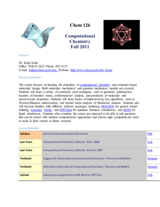
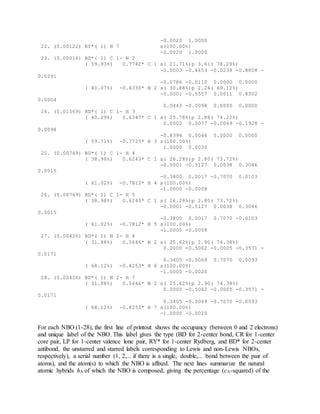
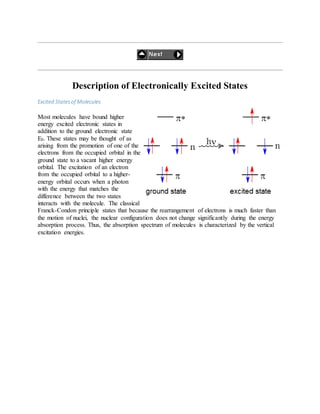
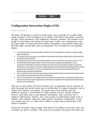
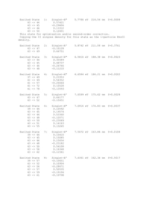
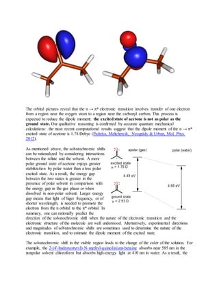
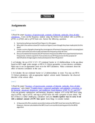
7. Finally, the natural populations are summarized as an effective valence electron configuration
("natural electron configuration") for each atom:
Atom # Natural Electron Configuration
----------------------------------------------------------------------------
C 1 [core]2s( 1.09)2p( 3.35)
N 2 [core]2s( 1.43)2p( 4.47)
H 3 1s( 0.81)
H 4 1s( 0.78)
H 5 1s( 0.78)
H 6 1s( 0.64)
H 7 1s( 0.64)
Although the occupancies of the atomic orbitals are non-integer in the molecular environment,
the effective atomic configurations can be related to idealized atomic states in "promoted"
configurations.
Natural Bond Orbital Analysis
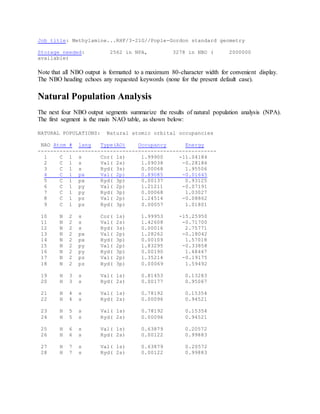
The next segments of the output summarize the results of NBO analysis. The first segment
reports on details of the search for an NBO natural Lewis structure:
NATURAL BOND ORBITAL ANALYSIS:
Occupancies Lewis Structure Low High
Occ. ------------------- ----------------- occ occ
Cycle Thresh. Lewis Non-Lewis CR BD 3C LP (L) (NL) Dev
=============================================================================
1(1) 1.90 17.95048 0.04952 2 6 0 1 0 0 0.02
-----------------------------------------------------------------------------
Structure accepted: No low occupancy Lewis orbitals
Normally, there is but one cycle of the NBO search. The table summarizes a variety of
information for each cycle: the occupancy threshold for a "good" pair in the NBO search; the
total populations of Lewis and non-Lewis NBOs; the number of core (CR), 2-center bond (BD),
3-center bond (3C), and lone pair (LP) NBOs in the natural Lewis structure; the number of low-
occupancy Lewis (L) and high-occupancy (> 0.1e) non-Lewis (NL) orbitals; and the maximum
deviation (Dev) of any formal bond order for the structure from a nominal estimate (NAO
Wiberg bond index). The Lewis structure is accepted if all orbitals of the formal Lewis structure
exceed the occupancy threshold (default = 1.90 electrons).
Next follows a more detailed breakdown of the Lewis and non-Lewis occupancies into core,
valence, and Rydberg shell contributions:
WARNING: 1 low occupancy (<1.9990e) core orbital found on C 1
--------------------------------------------------------
Core 3.99853 ( 99.963% of 4)
Valence Lewis 13.95195 ( 99.657% of 14)

8. ================== ============================
Total Lewis 17.95048 ( 99.725% of 18)
-----------------------------------------------------
Valence non-Lewis 0.03977 ( 0.221% of 18)
Rydberg non-Lewis 0.00975 ( 0.054% of 18)
================== ============================
Total non-Lewis 0.04952 ( 0.275% of 18)
--------------------------------------------------------
This shows the general quality of the natural Lewis structure description in terms of the
percentage of the total electron density (e.g., in the above case, about 99.7%). The table also
exhibits the relatively important role of the valence non-Lewis orbitals (i.e., the six valence
antibonds, NBOs 23-28, listed below) relative to the extra-valence orbitals (the 13 Rydberg
NBOs 10-22) in the slight departures from a localized Lewis structure model. The table also
includes a warning about a carbon core orbital with slightly less than double occupancy.
Next follows the main listing of NBOs, displaying the form and occupancy of the complete set of
orbitals that span the input AO space:
(Occupancy) Bond orbital/ Coefficients/ Hybrids
-----------------------------------------------------------------------------
--
1. (1.99858) BD ( 1) C 1- N 2
( 40.07%) 0.6330* C 1 s( 21.71%)p 3.61( 78.29%)
-0.0003 -0.4653 -0.0238 -0.8808 -
0.0291
-0.0786 -0.0110 0.0000 0.0000
( 59.93%) 0.7742* N 2 s( 30.88%)p 2.24( 69.12%)
-0.0001 -0.5557 0.0011 0.8302
0.0004
0.0443 -0.0098 0.0000 0.0000
2. (1.99860) BD ( 1) C 1- H 3
( 59.71%) 0.7727* C 1 s( 25.78%)p 2.88( 74.22%)
-0.0002 -0.5077 0.0069 0.1928
0.0098
0.8396 -0.0046 0.0000 0.0000
( 40.29%) 0.6347* H 3 s(100.00%)
-1.0000 -0.0030
3. (1.99399) BD ( 1) C 1- H 4
( 61.02%) 0.7812* C 1 s( 26.28%)p 2.80( 73.72%)
0.0001 0.5127 -0.0038 -0.3046 -
0.0015
0.3800 -0.0017 0.7070 -0.0103
( 38.98%) 0.6243* H 4 s(100.00%)
1.0000 0.0008
4. (1.99399) BD ( 1) C 1- H 5
( 61.02%) 0.7812* C 1 s( 26.28%)p 2.80( 73.72%)
0.0001 0.5127 -0.0038 -0.3046 -
0.0015
0.3800 -0.0017 -0.7070 0.0103
( 38.98%) 0.6243* H 5 s(100.00%)
1.0000 0.0008
5. (1.99442) BD ( 1) N 2- H 6
( 68.12%) 0.8253* N 2 s( 25.62%)p 2.90( 74.38%)

9. 0.0000 0.5062 0.0005 0.3571
0.0171
-0.3405 0.0069 -0.7070 -0.0093
( 31.88%) 0.5646* H 6 s(100.00%)
1.0000 0.0020
6. (1.99442) BD ( 1) N 2- H 7
( 68.12%) 0.8253* N 2 s( 25.62%)p 2.90( 74.38%)
0.0000 0.5062 0.0005 0.3571
0.0171
-0.3405 0.0069 0.7070 0.0093
( 31.88%) 0.5646* H 7 s(100.00%)
1.0000 0.0020
7. (1.99900) CR ( 1) C 1 s(100.00%)p 0.00( 0.00%)
1.0000 -0.0003 0.0000 -0.0002
0.0000
0.0001 0.0000 0.0000 0.0000
8. (1.99953) CR ( 1) N 2 s(100.00%)p 0.00( 0.00%)
1.0000 -0.0001 0.0000 0.0001
0.0000
0.0000 0.0000 0.0000 0.0000
9. (1.97795) LP ( 1) N 2 s( 17.85%)p 4.60( 82.15%)
0.0000 0.4225 0.0002 0.2360 -
0.0027
0.8749 -0.0162 0.0000 0.0000
10. (0.00105) RY*( 1) C 1 s( 1.57%)p62.84( 98.43%)
0.0000 -0.0095 0.1248 -0.0305
0.7302
-0.0046 0.6710 0.0000 0.0000
11. (0.00034) RY*( 2) C 1 s( 0.00%)p 1.00(100.00%)
0.0000 0.0000 0.0000 0.0000
0.0000
0.0000 0.0000 0.0146 0.9999
12. (0.00022) RY*( 3) C 1 s( 56.51%)p 0.77( 43.49%)
0.0000 -0.0023 0.7517 -0.0237
0.3710
-0.0094 -0.5447 0.0000 0.0000
13. (0.00002) RY*( 4) C 1 s( 41.87%)p 1.39( 58.13%)
14. (0.00116) RY*( 1) N 2 s( 1.50%)p65.53( 98.50%)
0.0000 -0.0062 0.1224 0.0063
0.0371
0.0197 0.9915 0.0000 0.0000
15. (0.00044) RY*( 2) N 2 s( 0.00%)p 1.00(100.00%)
0.0000 0.0000 0.0000 0.0000
0.0000
0.0000 0.0000 -0.0132 0.9999
16. (0.00038) RY*( 3) N 2 s( 33.38%)p 2.00( 66.62%)
0.0000 0.0133 0.5776 0.0087 -
0.8150
-0.0121 -0.0405 0.0000 0.0000
17. (0.00002) RY*( 4) N 2 s( 65.14%)p 0.54( 34.86%)
18. (0.00178) RY*( 1) H 3 s(100.00%)
-0.0030 1.0000
19. (0.00096) RY*( 1) H 4 s(100.00%)
-0.0008 1.0000
20. (0.00096) RY*( 1) H 5 s(100.00%)
-0.0008 1.0000
21. (0.00122) RY*( 1) H 6 s(100.00%)

10. -0.0020 1.0000
22. (0.00122) RY*( 1) H 7 s(100.00%)
-0.0020 1.0000
23. (0.00016) BD*( 1) C 1- N 2
( 59.93%) 0.7742* C 1 s( 21.71%)p 3.61( 78.29%)
-0.0003 -0.4653 -0.0238 -0.8808 -
0.0291
-0.0786 -0.0110 0.0000 0.0000
( 40.07%) -0.6330* N 2 s( 30.88%)p 2.24( 69.12%)
-0.0001 -0.5557 0.0011 0.8302
0.0004
0.0443 -0.0098 0.0000 0.0000
24. (0.01569) BD*( 1) C 1- H 3
( 40.29%) 0.6347* C 1 s( 25.78%)p 2.88( 74.22%)
0.0002 0.5077 -0.0069 -0.1928 -
0.0098
-0.8396 0.0046 0.0000 0.0000
( 59.71%) -0.7727* H 3 s(100.00%)
1.0000 0.0030
25. (0.00769) BD*( 1) C 1- H 4
( 38.98%) 0.6243* C 1 s( 26.28%)p 2.80( 73.72%)
-0.0001 -0.5127 0.0038 0.3046
0.0015
-0.3800 0.0017 -0.7070 0.0103
( 61.02%) -0.7812* H 4 s(100.00%)
-1.0000 -0.0008
26. (0.00769) BD*( 1) C 1- H 5
( 38.98%) 0.6243* C 1 s( 26.28%)p 2.80( 73.72%)
-0.0001 -0.5127 0.0038 0.3046
0.0015
-0.3800 0.0017 0.7070 -0.0103
( 61.02%) -0.7812* H 5 s(100.00%)
-1.0000 -0.0008
27. (0.00426) BD*( 1) N 2- H 6
( 31.88%) 0.5646* N 2 s( 25.62%)p 2.90( 74.38%)
0.0000 -0.5062 -0.0005 -0.3571 -
0.0171
0.3405 -0.0069 0.7070 0.0093
( 68.12%) -0.8253* H 6 s(100.00%)
-1.0000 -0.0020
28. (0.00426) BD*( 1) N 2- H 7
( 31.88%) 0.5646* N 2 s( 25.62%)p 2.90( 74.38%)
0.0000 -0.5062 -0.0005 -0.3571 -
0.0171
0.3405 -0.0069 -0.7070 -0.0093
( 68.12%) -0.8253* H 7 s(100.00%)
-1.0000 -0.0020
For each NBO (1-28), the first line of printout shows the occupancy (between 0 and 2 electrons)
and unique label of the NBO. This label gives the type (BD for 2-center bond, CR for 1-center
core pair, LP for 1-center valence lone pair, RY* for 1-center Rydberg, and BD* for 2-center
antibond, the unstarred and starred labels corresponding to Lewis and non-Lewis NBOs,
respectively), a serial number (1, 2,... if there is a single, double,... bond between the pair of
atoms), and the atom(s) to which the NBO is affixed. The next lines summarize the natural
atomic hybrids hA of which the NBO is composed, giving the percentage (cA-squared) of the

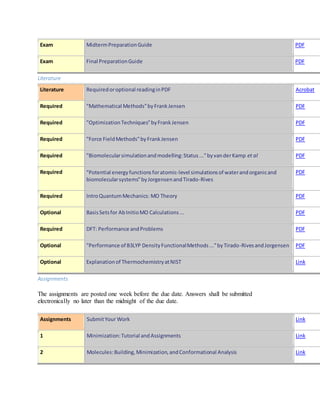
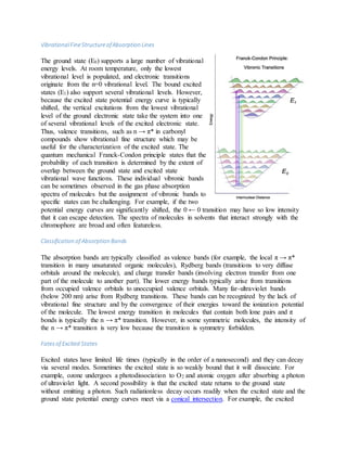
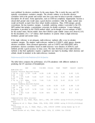
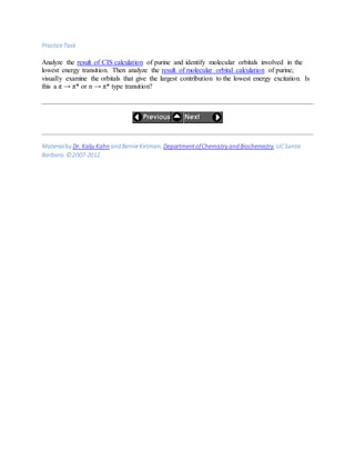
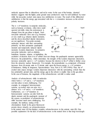
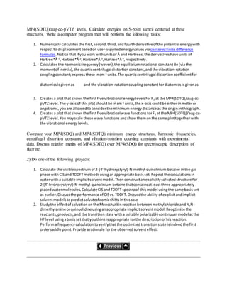
11. NBO on each hybrid (in parentheses), the polarization coefficient cA, the atom label, and a
hybrid label showing the sp-hybridization (percentage s-character, p-character, etc.) of each hA.
Below each NHO label is the set of coefficients that specify how the NHO is written explicitly as
a linear combination of NAOs on the atom. The order of NAO coefficients follows the
numbering of the NAO tables.
In the CH3NH2 example, the NBO search finds the C-N bond (NBO 1), three C-H bonds (NBOs
2, 3, 4), two N-H bonds (NBOs 5, 6), N lone pair (NBO 9), and C and N core pairs (NBOs 7, 8)
of the expected Lewis structure. NBOs 10-28 represent the residual non-Lewis NBOs of low
occupancy. In this example, it is also interesting to note the slight asymmetry of the three CH
NBOs, and the slightly higher occupancy (0.016 vs. 0.008 electrons) in the CH3 antibond (NBO
24) lying trans to the nitrogen lone pair.
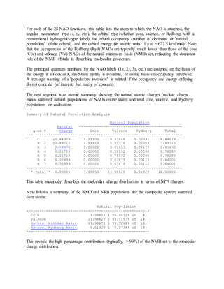
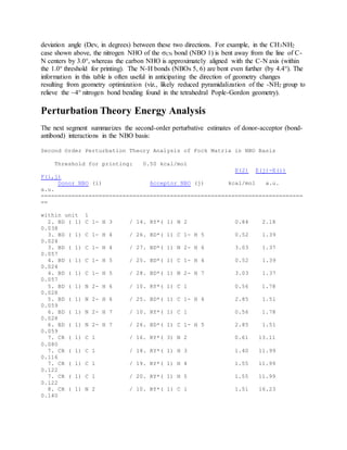
NHO Directional Analysis
The next segment of output summarizes the angular properties of the natural hybrid orbitals
(NHOs):
NHO Directionality and "Bond Bending" (deviations from line of nuclear
centers)
[Thresholds for printing: angular deviation > 1.0 degree]
hybrid p-character > 25.0%
orbital occupancy > 0.10e
Line of Centers Hybrid 1 Hybrid 2
--------------- ------------------- ----------------
--
NBO Theta Phi Theta Phi Dev Theta Phi
Dev
=============================================================================
==
1. BD ( 1) C 1- N 2 90.0 5.4 -- -- -- 90.0 182.4
3.0
3. BD ( 1) C 1- H 4 35.3 130.7 34.9 129.0 1.0 -- -- -
-
4. BD ( 1) C 1- H 5 144.7 130.7 145.1 129.0 1.0 -- -- -
-
5. BD ( 1) N 2- H 6 144.7 310.7 145.0 318.3 4.4 -- -- -
-
6. BD ( 1) N 2- H 7 35.3 310.7 35.0 318.3 4.4 -- -- -
-
9. LP ( 1) N 2 -- -- 90.0 74.8 -- -- -- -
-
The "direction" of a hybrid is specified in terms of the polar () and azimuthal () angles (in the
coordinate system of the calling program) of the vector describing its p-component. For more
general spd hybrids the hybrid direction is determined numerically to correspond to the
maximum angular amplitude. The hybrid direction is then compared with the direction of the line
of centers between the two nuclei to determine the bending of the bond, expressed as the

12. deviation angle (Dev, in degrees) between these two directions. For example, in the CH3NH2
case shown above, the nitrogen NHO of the CN bond (NBO 1) is bent away from the line of C-
N centers by 3.0°, whereas the carbon NHO is approximately aligned with the C-N axis (within
the 1.0° threshold for printing). The N-H bonds (NBOs 5, 6) are bent even further (by 4.4°). The
information in this table is often useful in anticipating the direction of geometry changes
resulting from geometry optimization (viz., likely reduced pyramidalization of the -NH2 group to
relieve the ~4° nitrogen bond bending found in the tetrahedral Pople-Gordon geometry).
Perturbation Theory Energy Analysis
The next segment summarizes the second-order perturbative estimates of donor-acceptor (bond-
antibond) interactions in the NBO basis:
Second Order Perturbation Theory Analysis of Fock Matrix in NBO Basis
Threshold for printing: 0.50 kcal/mol
E(2) E(j)-E(i)
F(i,j)
Donor NBO (i) Acceptor NBO (j) kcal/mol a.u.
a.u.
=============================================================================
==
within unit 1
2. BD ( 1) C 1- H 3 / 14. RY*( 1) N 2 0.84 2.18
0.038
3. BD ( 1) C 1- H 4 / 26. BD*( 1) C 1- H 5 0.52 1.39
0.024
3. BD ( 1) C 1- H 4 / 27. BD*( 1) N 2- H 6 3.03 1.37
0.057
4. BD ( 1) C 1- H 5 / 25. BD*( 1) C 1- H 4 0.52 1.39
0.024
4. BD ( 1) C 1- H 5 / 28. BD*( 1) N 2- H 7 3.03 1.37
0.057
5. BD ( 1) N 2- H 6 / 10. RY*( 1) C 1 0.56 1.78
0.028
5. BD ( 1) N 2- H 6 / 25. BD*( 1) C 1- H 4 2.85 1.51
0.059
6. BD ( 1) N 2- H 7 / 10. RY*( 1) C 1 0.56 1.78
0.028
6. BD ( 1) N 2- H 7 / 26. BD*( 1) C 1- H 5 2.85 1.51
0.059
7. CR ( 1) C 1 / 16. RY*( 3) N 2 0.61 13.11
0.080
7. CR ( 1) C 1 / 18. RY*( 1) H 3 1.40 11.99
0.116
7. CR ( 1) C 1 / 19. RY*( 1) H 4 1.55 11.99
0.122
7. CR ( 1) C 1 / 20. RY*( 1) H 5 1.55 11.99
0.122
8. CR ( 1) N 2 / 10. RY*( 1) C 1 1.51 16.23
0.140

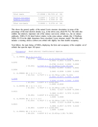
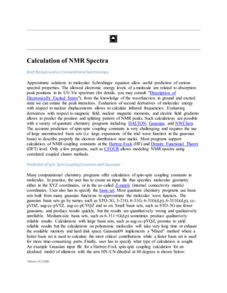
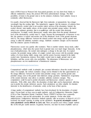
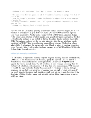
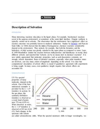
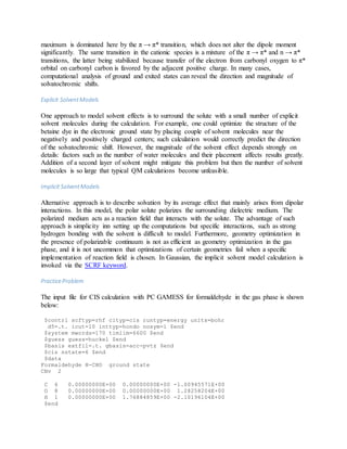
13. 8. CR ( 1) N 2 / 12. RY*( 3) C 1 0.84 16.77
0.106
8. CR ( 1) N 2 / 21. RY*( 1) H 6 0.61 16.26
0.089
8. CR ( 1) N 2 / 22. RY*( 1) H 7 0.61 16.26
0.089
9. LP ( 1) N 2 / 24. BD*( 1) C 1- H 3 8.13 1.13
0.086
9. LP ( 1) N 2 / 25. BD*( 1) C 1- H 4 1.46 1.14
0.037
9. LP ( 1) N 2 / 26. BD*( 1) C 1- H 5 1.46 1.14
0.037
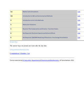
This analysis is carried out by examining all possible interactions between "filled" (donor)
Lewis-type NBOs and "empty" (acceptor) non-Lewis NBOs, and estimating their energetic
importance by 2nd-order perturbation theory. Since these interactions lead to donation of
occupancy from the localized NBOs of the idealized Lewis structure into the empty non-Lewis
orbitals (and thus, to departures from the idealized Lewis structure description), they are referred
to as "delocalization" corrections to the zeroth-order natural Lewis structure. For each donor
NBO (i) and acceptor NBO (j), the stabilization energy E(2) associated with delocalization ("2e-
stabilization") i  j is estimated as
where qi is the donor orbital occupancy, i, j are diagonal elements (orbital energies) and F(i,j)
is the off-diagonal NBO Fock matrix element. [In the example above, the nN  CH* interaction
between the nitrogen lone pair (NBO 8) and the antiperiplanar C1-H3 antibond (NBO 24) is seen
to give the strongest stabilization, 8.13 kcal/mol.] As the heading indicates, entries are included
in this table only when the interaction energy exceeds a default threshold of 0.5 kcal/mol.
NBO Summary
Next appears a condensed summary of the principal NBOs, showing the occupancy, orbital
energy, and the qualitative pattern of delocalization interactions associated with each:
Natural Bond Orbitals (Summary):
Principal Delocalizations
NBO Occupancy Energy (geminal,vicinal,remote)
=============================================================================
==
Molecular unit 1 (CH5N)
1. BD ( 1) C 1- N 2 1.99858 -0.89908
2. BD ( 1) C 1- H 3 1.99860 -0.69181 14(v)
3. BD ( 1) C 1- H 4 1.99399 -0.68892 27(v),26(g)
4. BD ( 1) C 1- H 5 1.99399 -0.68892 28(v),25(g)
5. BD ( 1) N 2- H 6 1.99442 -0.80951 25(v),10(v)

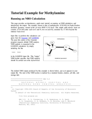
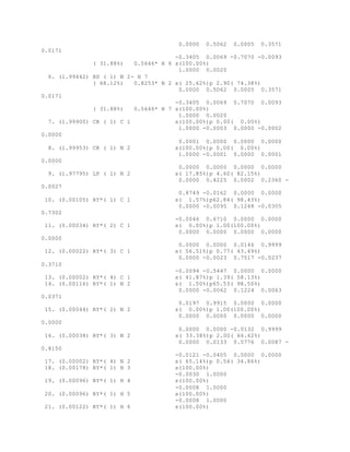
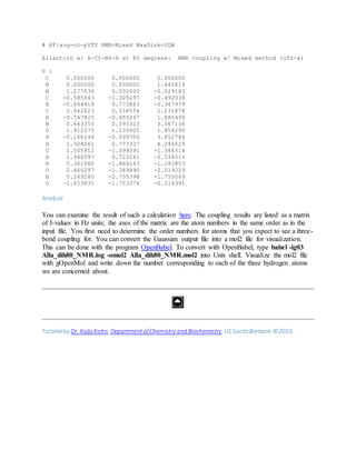
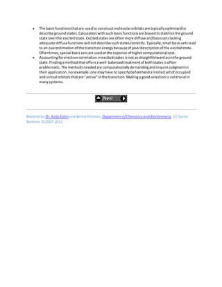
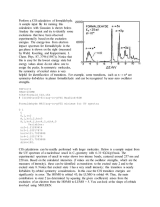
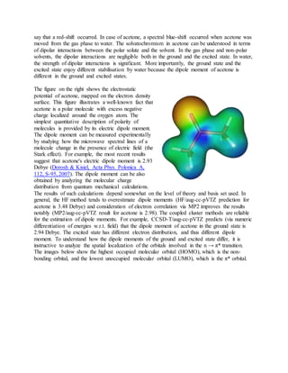
14. 6. BD ( 1) N 2- H 7 1.99442 -0.80951 26(v),10(v)
7. CR ( 1) C 1 1.99900 -11.04131 19(v),20(v),18(v),16(v)
8. CR ( 1) N 2 1.99953 -15.25927 10(v),12(v),21(v),22(v)
9. LP ( 1) N 2 1.97795 -0.44592 24(v),25(v),26(v)
10. RY*( 1) C 1 0.00105 0.97105
11. RY*( 2) C 1 0.00034 1.02120
12. RY*( 3) C 1 0.00022 1.51414
13. RY*( 4) C 1 0.00002 1.42223
14. RY*( 1) N 2 0.00116 1.48790
15. RY*( 2) N 2 0.00044 1.59323
16. RY*( 3) N 2 0.00038 2.06475
17. RY*( 4) N 2 0.00002 2.25932
18. RY*( 1) H 3 0.00178 0.94860
19. RY*( 1) H 4 0.00096 0.94464
20. RY*( 1) H 5 0.00096 0.94464
21. RY*( 1) H 6 0.00122 0.99735
22. RY*( 1) H 7 0.00122 0.99735
23. BD*( 1) C 1- N 2 0.00016 0.57000
24. BD*( 1) C 1- H 3 0.01569 0.68735
25. BD*( 1) C 1- H 4 0.00769 0.69640
26. BD*( 1) C 1- H 5 0.00769 0.69640
27. BD*( 1) N 2- H 6 0.00426 0.68086
28. BD*( 1) N 2- H 7 0.00426 0.68086
-------------------------------
Total Lewis 17.95048 ( 99.7249%)
Valence non-Lewis 0.03977 ( 0.2209%)
Rydberg non-Lewis 0.00975 ( 0.0542%)
-------------------------------
Total unit 1 18.00000 (100.0000%)
Charge unit 1 0.00000
This table allows one to quickly identify the principal delocalizing acceptor orbitals associated
with each donor NBO, and their topological relationship to this NBO, i.e., whether attached to
the same atom (geminal, "g"), to an adjacent bonded atom (vicinal, "v"), or to a more remote
("r") site. These acceptor NBOs will generally correspond to the principal "delocalization tails"
of the NLMO associated with the parent donor NBO. [For example, in the table above, the
nitrogen lone pair (NBO 9) is seen to be the lowest-occupancy (1.978 electrons) and highest-
energy (-0.446 a.u.) Lewis NBO, and to be primarily delocalized into antibonds 24, 25, 26 (the
vicinal CH NBOs). The summary at the bottom of the table shows that the Lewis NBOs 1-9
describe about 99.7% of the total electron density, with the remaining non-Lewis density found
primarily in the valence-shell antibonds (particularly, NBO 24).]
NBO Tutorials
NBO Home

15. Calculation of NMR Spectra
Brief Background on ComputationalSpectroscopy
Approximate solutions to molecular Schrodinger equation allow useful prediction of various
spectral properties. The allowed electronic energy levels of a molecule are related to absorption
peak positions in its UV-Vis spectrum (for details, you may consult "Description of
Electronically Excited States"); from the knowledge of the wavefunction in ground and excited
state we can estiate the peak intensities. Evaluation of second derivatives of molecular energy
with respect to nuclear displacements allows to calculate infrared frequencies. Evaluating
derivatives with respect to magnetic field, nuclear magnetic moments, and electric field gradients
allows to predict the position and splitting pattern of NMR peaks. Such calculations are possible
with a variety of quantum chemistry programs including DALTON, Gaussian, and NWChem.
The accurate prediction of spin-spin coupling constants is very challenging and requires the use
of large uncontracted basis sets (i.e. large expansions of the trial wave function in the gaussian
basis) to describe properly the electron distribution near nuclei. Most programs support
calculation of NMR coupling constants at the Hartree-Fock (HF) and Density Functional Theory
(DFT) level. Only a few programs, such as CFOUR allows modeling NMR spectra using
correlated coupled cluster methods.
Prediction ofSpin-Spin CouplingConstantswith Gaussian
Many computational chemistry programs offer calculation of spin-spin coupling constants in
molecules. In practice, the user has to create an input file that specifies molecular geometry
either in the XYZ coordinates, or in the so-called Z-matrix (internal connectivity matrix)
coordinates. User also has to specify the basis set. Most quantum chemistry programs use basis
sets built from many gaussian functions to approximate the molecular wave function. The
gaussian basis sets go by names such as STO-3G, 3-21G, 6-31G, 6-31G(d,p), 6-311G(d,p), cc-
pVDZ, aug-cc-pVTZ, aug-cc-pCVQZ and so on. Small basis sets, such as STO-3G use fewer
gaussians, and produce results quickly, but the results are quantitatively wrong and qualitatively
unreliable. Medium-size basis sets, such as 6-311+G(d,p) sometimes produce qualitatively
reliable results. Calculations with large basis sets, such as aug-cc-pVQZ, promise to yield
reliable results but the calculations on polyatomic molecules will take very long time or exhaust
the available memory and hard disk space. Gaussian09 implements a "Mixed" method where a
better basis set is used to calculate the most critical contributions while a faster basis set is used
for more time-consuming parts. Finally, user has to specify what type of calculation is sought.
An example Gaussian input file for a Hartree-Fock spin-spin coupling calculation for an
idealized model of allantoin with the arm HN-CN dihedral at 80 degrees is shown below:
%Mem=420MW

16. # HF/aug-cc-pVTZ NMR=Mixed MaxDisk=2GW
Allantoin w/ H-C5-N6-H at 80 degrees: NMR coupling w/ Mixed method (uTZ-w)
0 1
C 0.000000 0.000000 0.000000
N 0.000000 0.000000 1.445819
N 1.277036 0.000000 -0.629183
C -0.585043 -1.329297 -0.492038
H -0.664818 0.773863 -0.367979
C 0.942023 0.558554 2.231878
H -0.767825 -0.455267 1.880499
N 0.663355 0.393323 3.567138
O 1.912375 1.133905 1.854290
H -0.168148 -0.099700 3.852784
H 1.304261 0.773337 4.246029
C 1.505912 -1.098091 -1.386514
H 1.946597 0.723281 -0.534511
N 0.361060 -1.884143 -1.283853
O 2.466297 -1.369890 -2.019229
H 0.269280 -2.755398 -1.750049
O -1.653831 -1.753376 -0.214391
Analysis
You can examine the result of such a calculation here. The coupling results are listed as a matrix
of J-values in Hz units; the axes of the matrix are the atom numbers in the same order as in the
input file. You first need to determine the order numbers for atoms that you expect to see a three-
bond coupling for. You can convert the Gaussian output file into a mol2 file for visualization.
This can be done with the program OpenBabel. To convert with OpenBabel, type babel -ig03
Alla_dih80_NMR.log -omol2 Alla_dih80_NMR.mol2 into Unix shell. Visualize the mol2 file
with gOpenMol and write down the number corresponding to each of the three hydrogen atoms
we are concerned about.
Tutorialby Dr. Kalju Kahn, DepartmentofChemistry and Biochemistry, UCSanta Barbara. ©2010.

17. Description of Electronically Excited States
Excited Statesof Molecules
Most molecules have bound higher
energy excited electronic states in
addition to the ground electronic state
E0. These states may be thought of as
arising from the promotion of one of the
electrons from the occupied orbital in the
ground state to a vacant higher energy
orbital. The excitation of an electron
from the occupied orbital to a higher-
energy orbital occurs when a photon
with the energy that matches the
difference between the two states
interacts with the molecule. The classical
Franck-Condon principle states that because the rearrangement of electrons is much faster than
the motion of nuclei, the nuclear configuration does not change significantly during the energy
absorption process. Thus, the absorption spectrum of molecules is characterized by the vertical
excitation energies.

18. VibrationalFineStructureofAbsorption Lines
The ground state (E0) supports a large number of vibrational
energy levels. At room temperature, only the lowest
vibrational level is populated, and electronic transitions
originate from the n=0 vibrational level. The bound excited
states (E1) also support several vibrational levels. However,
because the excited state potential energy curve is typically
shifted, the vertical excitations from the lowest vibrational
level of the ground electronic state take the system into one
of several vibrational levels of the excited electronic state.
Thus, valence transitions, such as n → π* in carbonyl
compounds show vibrational fine structure which may be
useful for the characterization of the excited state. The
quantum mechanical Franck-Condon principle states that the
probability of each transition is determined by the extent of
overlap between the ground state and excited state
vibrational wave functions. These individual vibronic bands
can be sometimes observed in the gas phase absorption
spectra of molecules but the assignment of vibronic bands to
specific states can be challenging. For example, if the two
potential energy curves are significantly shifted, the 0 ← 0 transition may have so low intensity
that it can escape detection. The spectra of molecules in solvents that interact strongly with the
chromophore are broad and often featureless.
Classification of Absorption Bands
The absorption bands are typically classified as valence bands (for example, the local π → π*
transition in many unsaturated organic molecules), Rydberg bands (transitions to very diffuse
orbitals around the molecule), and charge transfer bands (involving electron transfer from one
part of the molecule to another part). The lower energy bands typically arise from transitions
from occupied valence orbitals to unoccupied valence orbitals. Many far-ultraviolet bands
(below 200 nm) arise from Rydberg transitions. These bands can be recognized by the lack of
vibrational fine structure and by the convergence of their energies toward the ionization potential
of the molecule. The lowest energy transition in molecules that contain both lone pairs and π
bonds is typically the n → π* transition. However, in some symmetric molecules, the intensity of
the n → π* transition is very low because the transition is symmetry forbidden.
Fatesof Excited States
Excited states have limited life times (typically in the order of a nanosecond) and they can decay
via several modes. Sometimes the excited state is so weakly bound that it will dissociate. For
example, ozone undergoes a photodissociation to O2 and atomic oxygen after absorbing a photon
of ultraviolet light. A second possibility is that the excited state returns to the ground state
without emitting a photon. Such radiationless decay occurs readily when the excited state and the
ground state potential energy curves meet via a conical intersection. For example, the excited

19. states of DNA bases in Watson-Crick base paired geometry are very short-lived thanks to
efficient radiationless decay; this protects DNA from photochemical damage. The third
possibility of return to the ground state is via the emission of photon. Such radiative decay is
commonly called fluorescence.
It is usually observed that the fluorescent light from molecules or nanoparticles has a longer
wavelength than the exciting light. This immediately suggests that the emission of a photon from
the electronically excited state is not a perfect mirror process of the absorption. Instead, the
excited vibronic state rapidly relaxes on the excited state potential energy surface: the nuclei
adopt a new optimum geometry that is at equilibrium with the excited state electronic
wavefunction. In simple words, fluorescence usually takes place from the ground vibrational
level of the electronically excited state E1. Again, because the rearrangement of electrons is very
fast, the emission is vertical and reaches one of the vibrational levels of the ground electronic
state E0. The energy difference between the relaxed excited state energy and the ground state
energy is called the adiabatic excitation energy. Adiabatic excitation energies can be measured
from the emission spectra of molecules.
Fluorescence occurs very quickly after excitation. There is another radative decay mode, called
phosphoresence, which takes the system back to ground state over much longer timescales. In the
case of phosphoresence, the excited state undergoes a change in the spin state. In a typical
scenario, the potential energy surface of a singlet excited state crosses with the potential energy
surface of a lower-laying triplet energy state, and the system becomes trapped in the triplet
excited state. Spontaneous emission from triplet excited state to singlet ground state is spin
forbidden, and thus occurs with a low probability. The phenomena of fluorescence and
phosphoresence are two manifestations of luminescent emission.
ComputationalMethodsforExcited States
Computational methods could, in principle give accurate information about the excited electronic
states. For example, the vertical excitation energy can be obtained in the first approximation as
the energy difference between the excited state potential energy curve and the ground state
potential energy curve at the ground state minimum energy geometry. Optimization of geometry
of the excited electronic state allows to calculate adiabatic excitation energies. Thus,
computations could be used to predict absorption and fluorescence emission spectra of
molecules. With a little more effort, the absorption of chiral light can be characterized, allowing
one to predict the circular dichroism spectra. Such calculations are often valuable for chemists
interested in the identification of molecules solely on the basis of their spectra.
A large number of computational methods have been developed for the description of excited
states. On one hand, we have easy-to-apply methods, such as Configuration Interaction Singles
(CIS) or Time Dependent Density Functional Theory (TDDFT) but these have a generally
limited accuracy, and can fail spectacularly for certain situations. On the other hand,
multireference configuration interaction methods typically offer an accuracy of about 0.1 eV (2.3
kcal/mol) but require expertise in setting up the calculation. In general, meaningful excited
state calculations can be difficult to carry out. There are special cases where a simple method
like (CIS) will give useful answers. In general, however, one must be aware of pitfalls such as:

20.  The basisfunctionsthatare usedto constructmolecularorbitalsare typicallyoptimizedto
describe groundstates.Calculationwithsuchbasisfunctionsare biasedtostabilizethe ground
state overthe excitedstate.Excitedstatesare oftenmore diffuse andbasissetslacking
adequate diffusefunctionswill notdescribesuchstatescorrectly.Typically,small basissetslead
to an overestimationof the transitionenergybecauseof poordescriptionof the excitedstate.
Oftentimes,special basissetsare usedatthe expense of highercomputationalcost.
 Accountingforelectroncorrelationinexcitedstatesisnot asstraightforwardasinthe ground
state.Findingamethodthatoffersa well-balancedtreatmentof bothstatesisoften
problematic.The methodsneededare computationallydemandingandrequire judgmentin
theirapplication.Forexample,one mayhave to specifybeforehandalimitedsetof occupied
and virtual orbitalsthatare "active"inthe transition.Makinga goodselectionisnottrivial in
manysystems.
Materialby Dr. Kalju Kahn and BernieKirtman, DepartmentofChemistry and Biochemistry, UCSanta
Barbara. ©2007-2012.

21. Configuration Interaction Singles (CIS)
BackgroundaboutCIS
The simple CIS approach is accurate in certain special cases, in particular for so-called charge
transfer transitions. In the CIS approach we use orbitals of the Hartree-Fock solution to generate
all singly excited determinants of the configuration interaction expansion. This treatment can be
thought of as the Hartree-Fock method for excited states. It allows one to simultaneously solve
for a large number of excited states and to optimize the geometry of any (desired) selected state.
Both spin singlet and spin triplet states can be generated. The CIS method has some appealing
features:
 It isrelativelyfastcomparedtoothermethods;CIScanbe appliedtosystemsaslarge as DNA
duplex oligomers.
 It iseasyto set up;typically,the numberof desiredexcitedstatesandthe basissetare the only
quantitiestobe specified.
 It ispossible todiscussthe electronictransitionsintermsof familiarconcepts,suchasπ → π*.
 CIS allowsgeometryoptimizationof the excitedstate usinganalyticalgradients.Thus,
calculationof adiabaticexcitationenergiesaswell asvertical excitationenergiesispractical.
Propertiessuchasdipole moments,charge densities,andvibrational frequenciesof the excited
statescan be calculated.Fromthe suchpropertiesone cancompare bondingdifferences
betweengroundandexcitedstates.
 CIS isvariational;the lowestenergysolutioncorrespondstothe groundelectronicstate andthe
nextsolutioncorrespondstothe firstexcitedstate.
 CIS issize-consistent;one willgetthe same excitationenergywhenconsidering asingle helium
atom or twoheliumatomsseparatedbyadistance so large that the weakinteractionbetween
atomscan be neglected.
There are two main problem with the CIS method. First, it is appropriate only for transitions for
which the ground state and the excited state are well-described by a single-configuration (such as
Hartree-Fock) reference wave function. The ground state of most molecules near their
equilibrium geometry is well described by a single reference (ozone is a notable exception).
However, some exited states in many important chromophores (such as benzene) have a
significant multi-reference character. Also, a close spacing on d-shell electron energy levels in
transition metal complexes means that a single-reference description is inappropriate. In such
cases, typical errors are 1 eV, which makes it difficult to assign observed spectral lines in the
absence of symmetry.
Second, the CIS method, being an analog of the Hartree-Fock method for the excited states, does
not include any electron correlation. This would not be a problem if the ground and excited state

22. were stabilized by electron correlation by the same degree. This is rarely the case, and CIS
typically overestimates excitation energies. The obvious solution is to describe electron
correlation both in the ground and excited state but a care must be taken to provide a balanced
description for all states. Some approaches, such as CISD are completely inappropriate because a
closed-shell ground state would enjoy a good electron correlation while the singly excited state
would not benefit as much from from virtual double excitations. Thus, CISD energies grossly
overestimate the true transition energies. A partially satisfying solution is provided in the CIS-
MP2 method that includes a perturbation correction for double excitations. A more balanced
description is provided by the CIS(D) method which can be thought of as an analogue of MP2
for the excited states. Recent studies show that CIS(D) is quite reliable (mean error about 0.2 eV)
for the description of n → π* valence shell transitions in systems where a single-reference
dominates ground and excited states.
If the single reference is not adequate, multi-reference methods offer a way to calculate
excitation energies. The simplest multi-reference method is CASSCF, which ignores dynamic
electron correlation. More advanced approaches, such as CASPT2 and XMCQDPT add a
perturbative electron correlation based on multi-reference wave function (CASSCF); such
methods provide a good accuracy in many cases. The main drawback of such multi-reference
methods is that their application requires a significant user input by deciding which electrons and
orbitals should be included in the multi-reference treatment.
PerformanceofCIS in the Prediction ofUV-VisSpectra
The table below compares the performance of a CIS calculation with different methods in
predicting the UV spectrum of formaldehyde:
EXP CIS CIS-MP2 CIS(D) TDHF TDDFT CASSCF CASPT2
EOM-CCSD CC3
Singlet Valence Excited States
1 1A2 (n → π*) 3.79* 4.48 4.58 3.98 4.35 3.92 4.62 3.91
4.04 3.88
1 1B1 (σ → π*) 8.68 9.66 8.47 8.12 9.52 9.03 6.88 9.09
9.26 9.04
2 1A1 (π → π*) NObs 9.36 7.66 7.26 9.55 8.43 10.24 9.77
10.0 9.18
Singlet Rydberg Excited States
1 1B2 (n → 3s) 7.11 8.63 6.85 6.44 8.59 6.87 6.88 7.30
7.04 N/A
2 1A2 (n → 3p) 8.37 9.78 7.83 7.50 9.74 7.89 8.17 8.32
8.21 8.21
2 1B2 (n → 4s) 9.26 10.8 8.94 N/A N/A N/A N/A N/A
9.35 N/A
Computational data sources:
Gwaltney et al, Chem. Phys. Lett., 248, 189 (1996) using 6-311(2+,2+)G(d,p)
basis
Wiberg et al J. Phys. Chem. 106, 4192, 2002 (2008) using 6-311(2+,2+)G(d,p)
basis
Schreiber et al, J. Chem. Phys., 128, 134110 (2008) using bases up to d-
aug-cc-pVTZ
Head-Gordon et al, Chem. Phys. Lett. 219, 21 (1994) for CIS(D)

23. Sunanda et al, Spectrosc. Lett. 45, 65 (2011) for some CIS data
* The estimates for the position of 0-0 vertical transition range from 3.5 eV
to 4.2 eV.
This forbidden transition is seen in absorption spectra as a broad system
of peaks due
to many vibrational transitions. Analogous vibrational structure is also
seen in the
energy loss spectra from electron impact.
Note that while the CIS method generally overestimates vertical ionization energies, the n → π*
transition in formaldehyde is given fairly well by the CIS, and the MP2 correction improves
some results considerably. Another method similar to CIS is TDHF (time-dependent Hartree-
Fock), which is a modification of CIS to include some ground state electron correlation. The last
of the affordable and easy-to-use methods is the time-dependent density functional theory (TD-
DFT). This methods performs well for low-lying electronic states that are not charge transfer
transitions but TD-DFT fails to model excited states of linear polyenes. The last four columns
refer to higher level methods that are generally more difficult to set up, or very time-consuming
to run. Currently, higher level wavefunction-based methods (e.g. CASPT2 or EOM-CCSD) offer
the best choice for small molecules.
Running and Analyzing CIS Calculations
The CIS method is implemented in many computer programs including Gaussian and Firefly (PC
GAMESS). To run the calculation with Gaussian, specify the keyword CIS. The number of
desired excited states can be specified as an option to the CIS keyword: CIS(NStates=8)
requests the 8 lowest excited states. The CIS calculation is more resource-consuming than the
Hartree-Fock calculation, and calculations with large basis sets, such as aug-cc-pVTZ, may not
be possible for larger molecules. Smaller basis such as 6-31+G(d) may be feasible for larger
molecules, but one shall worry about loss of accuracy when too small of a basis set is used. If
one is only interested in valence-shell transitions, small basis sets can be used. However, for the
description of diffuse Rydberg states, basis sets with multiple diffuse functions (e.g. d-aug-cc-
pVTZ) are critical.

24. Perform a CIS calculation of formaldehyde.
A sample input file for running this
calculation with Gaussian is shown below.
Analyze the output and try to identify some
excitations that have been observed
experimentally based on the excitation
energies. The energy-loss from electron
impact spectrum for formaldehyde in the
gas phase is shown on the right (measured
by Walzl, Koerting, and Kuppermann; J.
Chem. Phys. 87, 3796 (1987)). Notice that
this is easy for the lowest energy state but
energy values alone do not allow one to
assign the peaks. In symmetric molecules,
the symmetry of excited states is very
helpful for identification of transitions. For example, some transitions, such as n → π* are
symmetry-forbidden in planar formaldehyde and can be recognized by near-zero oscillator
strengths.
%NProc=1
%Mem=200MW
%Chk=Formald_CIS.chk
# CIS(NStates=6)/aug-cc-pVTZ MaxDisk=4GW
Formaldehyde MP2/aug-cc-pVTZ minimum for UV spectra
0 1
C
O,1,oc2
H,1,hc3,2,hco3
H,1,hc4,2,hco4,3,dih4,0
Variables:
oc2=1.21289414
hc3=1.10017879
hco3=121.7009888
hc4=1.10017879
hco4=121.7009888
dih4=180.
CIS calculations can be readily performed with larger molecules. Below is a sample output from
the UV spectrum of a nucleobase uracil in Cs geometry with 6-31+G(2d,p) basis. The
experimental spectrum of uracil in water shows two intense bands, centered around 257 nm and
220 nm. Based on the calculated intensities (f values are the oscillator strengths, which are the
measures of intensity), these can be identified as transitions to the excited state 2 and to the
excited state 8. Notice that excited state 1 has a very small intensity: this transition is nearly
forbidden by orbital symmetry considerations. In this case the CIS transition energies are
significantly in error. The HOMO is orbital 43; the LUMO is orbital 44. Thus, the main
contribution to state 2 (as determined by squaring the given coefficient) arises from the
excitation of an electron from the HOMO to LUMO + 5. You can look at the shape of orbitals
involved using MOLDEN.

25. Excited State 1: Singlet-A" 5.7786 eV 214.56 nm f=0.0008
43 -> 44 0.57421
43 -> 45 -0.29806
43 -> 46 0.13312
43 -> 50 0.12401
This state for optimization and/or second-order correction.
Copying the CI singles density for this state as the 1-particle RhoCI
density.
Excited State 2: Singlet-A' 5.8742 eV 211.06 nm f=0.3761
43 -> 47 -0.10128
43 -> 49 0.66751
Excited State 3: Singlet-A" 6.5816 eV 188.38 nm f=0.0023
43 -> 44 0.35589
43 -> 45 0.48737
43 -> 46 -0.24746
43 -> 48 -0.11210
Excited State 4: Singlet-A" 6.6584 eV 186.21 nm f=0.0002
37 -> 49 0.23353
41 -> 49 0.54352
41 -> 57 -0.20644
41 -> 72 0.10528
41 -> 78 -0.13593
Excited State 5: Singlet-A' 7.0599 eV 175.62 nm f=0.0028
43 -> 47 0.66177
43 -> 52 -0.15451
Excited State 6: Singlet-A" 7.0916 eV 174.83 nm f=0.0037
39 -> 44 0.10592
43 -> 45 0.19574
43 -> 46 0.53360
43 -> 48 -0.12071
43 -> 50 -0.23089
43 -> 51 0.16163
43 -> 55 0.13265
Excited State 7: Singlet-A" 7.5672 eV 163.84 nm f=0.0108
39 -> 44 0.10410
43 -> 45 0.15085
43 -> 46 0.15656
43 -> 48 -0.23182
43 -> 50 0.54108
43 -> 56 0.16348
43 -> 62 -0.11541
Excited State 8: Singlet-A' 7.6361 eV 162.36 nm f=0.5017
39 -> 57 -0.10651
43 -> 52 0.10904
43 -> 54 -0.28671
43 -> 57 0.50535
43 -> 59 -0.19194
43 -> 61 -0.19798

26. PracticeTask
Analyze the result of CIS calculation of purine and identify molecular orbitals involved in the
lowest energy transition. Then analyze the result of molecular orbital calculation of purine;
visually examine the orbitals that give the largest contribution to the lowest energy excitation. Is
this a π → π* or n → π* type transition?
Materialby Dr. Kalju Kahn and BernieKirtman, DepartmentofChemistry and Biochemistry, UCSanta
Barbara. ©2007-2012.

27. Description of Solvation
Introduction
Many interesting reactions take place in the liquid phase. For example, biochemical reactions
occur in the aqueous environment or sometimes at the water-lipid interface. Organic synthesis is
typically carried out in solvents. The observation that the environment has a significant effect on
reaction outcomes was probably known to medieval alchemists. Studies by Berhelot and Pean de
Saint Gilles in 1860s showed that the rates of homogeneous chemical reactions considerably
depend on the environment. They noticed, for example, that both the formation and the
hydrolysis of ethyl acetate was greatly retarded in the vapor phase as compared to water. Later,
in 1890 Menshutkin studied the reaction between trialkylamines and haloalkanes in twenty three
different solvents and reported that "solvents are by no means inert in chemical reactions". It is
now widely appreciated that molecular properties, such as acid dissociation constants, are
strongly solvent dependent. Rates of chemical reactions, especially when polar transition states
are involved, can vary many orders of magnitude depending on the solvent. It is clear that
computational description of solvent effects is crucial if quantitative agreement with experiments
is being sought. In many cases, even qualitative insight requires that solvent effects are
accounted for.
Solvatochromism
UV-Vis spectral
properties of many
molecules depend on the
solvent. One of the best
understood examples is
provided by the n → π*
transition in acetone. In
the gas phase, this
symmetry-forbidden
transition is observed as
a weak band of peaks
near 276 nm (4.49 ev).
When dissolved in water,
the n → π* transition is
observed at 265 nm (4.68
eV). Such changes in the
spectrum with solvent
are called solvatochromic shifts. When the spectral maximum shifts to longer wavelengths, we

28. say that a red-shift occurred. In case of acetone, a spectral blue-shift occurred when acetone was
moved from the gas phase to water. The solvatochromism in acetone can be understood in terms
of dipolar interactions between the polar solute and the solvent. In the gas phase and non-polar
solvents, the dipolar interactions are negligible both in the ground and the excited state. In water,
the strength of dipolar interactions is significant. More importantly, the ground state and the
excited state enjoy different stabilisation by water because the dipole moment of acetone is
different in the ground and excited states.
The figure on the right shows the electrostatic
potential of acetone, mapped on the electron density
surface. This figure illustrates a well-known fact that
acetone is a polar molecule with excess negative
charge localized around the oxygen atom. The
simplest quantitative description of polarity of
molecules is provided by its electric dipole moment.
The dipole moment can be measured experimentally
by studying how the microwave spectral lines of a
molecule change in the presence of electric field (the
Stark effect). For example, the most recent results
suggest that acetone's electric dipole moment is 2.93
Debye (Dorosh & Kisiel, Acta Phys. Polonica A,
112, S-95, 2007). The dipole moment can be also
obtained by analyzing the molecular charge
distribution from quantum mechanical calculations.
The results of such calculations depend somewhat on the level of theory and basis set used. In
general, the HF method tends to overestimate dipole moments (HF/aug-cc-pVTZ prediction for
acetone is 3.48 Debye) and consideration of electron correlation via MP2 improves the results
notably (MP2/aug-cc-pVTZ result for acetone is 2.98). The coupled cluster methods are reliable
for the estimation of dipole moments. For example, CCSD-T/aug-cc-pVTZ predicts (via numeric
differentiation of energies w.r.t. field) that the dipole moment of acetone in the ground state is
2.94 Debye. The excited state has different electron distribution, and thus different dipole
moment. To understand how the dipole moments of the ground and excited state differ, it is
instructive to analyze the spatial localization of the orbitals involved in the n → π* transition.
The images below show the highest occupied molecular orbital (HOMO), which is the non-
bonding orbital, and the lowest unoccupied molecular orbital (LUMO), which is the π* orbital.

29. The orbital pictures reveal that the n → π* electronic transition involves transfer of one electron
from a region near the oxygen atom to a region near the carbonyl carbon. This process is
expected to reduce the dipole moment: the excited state of acetone is not as polar as the
ground state. Our qualitative reasoning is confirmed by accurate quantum mechanical
calculations: the most recent computational results suggest that the dipole moment of the n → π*
excited state of acetone is 1.78 Debye (Pašteka, Melichercík, Neogrády & Urban, Mol. Phys.
2012).
As mentioned above, the solvatochromic shifts
can be rationalized by considering interactions
between the solute and the solvent. A more
polar ground state of acetone enjoys greater
stabilization by polar water than a less polar
excited state. As a result, the energy gap
between the two states is greater in the
presence of polar solvent in comparison with
the energy gap in the gas phase or when
dissolved in non-polar solvent. Larger energy
gap means that light of higer frequency, or of
shorter wavelength, is needed to promote the
electron from the n orbital to the π* orbital. In
summary, one can rationally predict the
direction of the solvatochromic shift when the nature of the electronic transition and the
electronic structure of the molecule are well understood. Alternatively, experimental directions
and magnitudes of solvatochromic shifts are sometimes used to determine the nature of the
electronic transition, and to estimate the dipole moment of the excited state.
The solvatochromic shift in the visible region leads to the change of the color of the solution. For
example, the 2-(4'-hydroxystyryl)-N-methyl-quinolinium-betaine absorbs near 585 nm in the
nonpolar solvent chloroform but absorbs high-energy light at 410 nm in water. As a result, the

30. molecule appears blue in chloroform and red in water. In the case of the betaine, chemical
intuition suggests that the highly polar ground state (zwitterion!) must be well stabilized by water
while the non-polar excited state enjoys less stabilization in water. The result of this differential
stabilization is that the energy gap associated with the n → π transition increases as the solvent
polarity increases.
The π → π* transitions in nonpolar molecules,
such as benzene or toluene, often show small
spectral red-shifts when the environment is
changed from the gas phase to liquid. Such
non-polar molecules have zero (e.g. benzene)
or very small (e.g. toluene) dipole moments,
and the above-described dipolar interactions
are not significant. Non-polar aromatic
molecules interact with their surrounding
primarily via their permanent quadrupole
moment and temporarily induced dipole
moments (London dispersion). In symmetric
non-polar molecules such as ethylene,
butadiene, benzene, toluene, or naphtalene, the
excitation of electron from π to π* orbital does not change the quadrupole moment appreciably.
However, the polarizability, which determines the strength of the London dispersion interaction,
increases noticeably upon π → π* excitation because the electron in the π* orbital is farther away
from the attractive nuclear framework. For example, the perpendicular αzz component of benzene
increases from 44 atomic units to 52 atomic units upon the lowest-energy π → π* excitation
(Christiansen, Hättig & Jørgensen, Spectrochimica Acta, Part A 55, 509 (1999)). Thus, the π*
excited state enjoys stronger London dispersion interaction with the surrounding solvent than the
less polarizable ground state, and the energy gap in the solvent is smaller than in the gas phase.
In the case of benzene, the magnitude of the solvatochromic red shift is rather small.
Analysis of solvatochromic shifts in molecules
where both π → π* and n; → π* transitions
can take place is more challenging. For
example, in conjugated heteroaromatic
systems, an excited state can arise via a
mixture of π → π* and n; → π* transitions.
Furthermore, a π → π* transition in
heteroaromatic systems can alter both the
dipole moment and the quadrupole moment of
the system, so prediction of solvatochromic
shifts becomes much more challenging. For
example, the methoxy analog of the
chromophore found in the green fluorescent
protein shows virtually no solvatochromisms
in the neutral state (A) but displays complex solvatochromism in the cationic state (B). One
possible explanation for the lack of solvatochromism in the neutral form is that long-wavelength

31. maximum is dominated here by the π → π* transition, which does not alter the dipole moment
significantly. The same transition in the cationic species is a mixture of the π → π* and n → π*
transitions, the latter being stabilized because transfer of the electron from carbonyl oxygen to π*
orbital on carbonyl carbon is favored by the adjacent positive charge. In many cases,
computational analysis of ground and exited states can reveal the direction and magnitude of
solvatochromic shifts.
Explicit SolventModels
One approach to model solvent effects is to surround the solute with a small number of explicit
solvent molecules during the calculation. For example, one could optimize the structure of the
betaine dye in the electronic ground state by placing couple of solvent molecules near the
negatively and positively charged centers; such calculation would correctly predict the direction
of the solvatochromic shift. However, the magnitude of the solvent effect depends strongly on
details: factors such as the number of water molecules and their placement affects results greatly.
Addition of a second layer of solvent might mitigate this problem but then the number of solvent
molecules is so large that typical QM calculations become unfeasible.
Implicit SolventModels
Alternative approach is to describe solvation by its average effect that mainly arises from dipolar
interactions. In this model, the polar solute polarizes the surrounding dielectric medium. The
polarized medium acts as a reaction field that interacts with the solute. The advantage of such
approach is simplicity inn setting up the computations but specific interactions, such as strong
hydrogen bonding with the solvent is difficult to model. Furthermore, geometry optimization in
the presence of polarizable continuum is not as efficient as geometry optimization in the gas
phase, and it is not uncommon that optimizations of certain geometries fail when a specific
implementation of reaction field is chosen. In Gaussian, the implicit solvent model calculation is
invoked via the SCRF keyword.
PracticeProblem
The input file for CIS calculation with PC GAMESS for formaldehyde in the gas phase is shown
below:
$contrl scftyp=rhf cityp=cis runtyp=energy units=bohr
d5=.t. icut=10 inttyp=hondo nosym=1 $end
$system mwords=170 timlim=6600 $end
$guess guess=huckel $end
$basis extfil=.t. gbasis=acc-pvtz $end
$cis nstate=6 $end
$data
Formaldehyde H-CHO ground state
CNv 2
C 6 0.00000000E+00 0.00000000E+00 -1.00945571E+00
O 8 0.00000000E+00 0.00000000E+00 1.28258204E+00
H 1 0.00000000E+00 1.76884859E+00 -2.10196104E+00
$end

32. Run this by issuing pcgamess -f -i form_cis.inp -o form_cis.out -b /usr/local/pcgamess/acc-
pvtz.lib. Examine the output file with a text editor and with MOLDEN to identify orbitals
involved in the lowest energy forbidden transition. Then build a formaldehyde water complex;
keep the structure of formaldehyde and water fixed and calculate the CIS spectrum of the
complex. Interpret the results.
Tutorialby Dr. Kalju Kahn, DepartmentofChemistry and Biochemistry, UCSanta Barbara. �2008-2012

33. Assignments
Level 1
1) Read the paper Accuracy of spectroscopic constants of diatomic molecules from ab initio
calculations . Carry out the frequency analysis using the Hartree Fock method with cc-pVDZ, cc-
pVTZ, cc-pVQZ, and cc-pV5Z basis sets. Answer the following questions.
1. Summarize whatyoulearnedfromFigure 1in thispaper.
2. Why didn'tthe authorsshowSCF resultsonFigure 2 eventhoughtheyhave made plotsforthis
data?
3. Create a seriesof graphsshowingthe convergence of harmonicfrequencywithincreasingbasis
setfor eachmolecule andvisuallyestimate the frequencyatthe HFlimit.
4. Discussfundamental reasonswhyHFharmonicfrequenciesdifferfromexperimental harmonic
frequencies.Isthere aquickfix if one wishestouse HFfrequenciesforthe purpose of
identificationof large organicmoleculesbasedontheirIRspectra?
2. a) Calculate the syn (Cl-C–C-Cl = 0°) rotational barrier in 1,2-dichloroethane in the gas phase
based on MP3 single point energies at HF/6-31+G(d,p) geometries to treat electron correlation.
Make sure to use an appropriate basis set in the MP3 calculation. Make a statement about the
effect of electron correlation in this case.
2. b) Calculate the syn rotational barrier in 1,2-dichroroethane in water. You may use HF/6-
31+G(d,p) calculations with an appropriate implicit solvent model. Rationalize the observed
direction of the solvent effect.
Level 2
1) Read the paper "Accuracy of spectroscopic constants of diatomic molecules from ab initio
calculations" and a paper "Coupled-cluster connected quadruples and quintuples corrections to
the harmonic vibrational frequencies and equilibrium bond distances of HF, N2, F2, and CO".
Carry out geometry optimization and harmonic frequency analysis of F2 at the MP3 level using
aug-cc-pVDZ, aug-cc-pVTZ, and aug-cc-pVQZ basis sets with a program of your choice. The
last of these is a rather challenging calculation and you should expolore ways to carry it out
with a minimal amount of CPU time spent. Some things to consider include:
1. 1) Gaussian03 offersanalyticsecondderivativesatthe MP2 level butnotatthe MP3 level.
However,Hessiancalculatedatthe MP2 level isanexcellentstartingpointforthe BFGS
algorithm

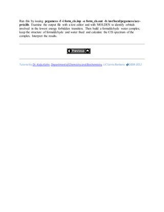
34. 2. 2) Gaussianoffersanalyticfirstderivativesatthe MP3 level.Secondderivativesatthe MP3 level
inGaussianare evaluatedbynumericdifferentiationof analyticfirstderivatives.
3. 3) PC GAMESS doesnot allowautomatedgeometryoptimizationorfrequencyanalysisatthe
MP3 level butoffersextremelyfastsingle pointMP3energies.
4. 4) Numericdifferentiationrequiresratheraccurate energyvalues.WithPCGAMESS / Firefly,the
followingperformance andaccuracy-relatedoptionsare recommended:
$contrl icut=10 inttyp=hondo$end
$systemmwords=60 $end$scf nconv=7 $end$mp3 cutoff=1E-14 $end
5. 5) Speedof electroncorrelationcalculationswithPCGAMESSdependsonthe choice between
the the conventional ($scf direct=.f.$end) anddirect($scf direct=.t.$end) methodforthe SCF
part. If you have a veryfast disk,itisbetterto write the atomicintegralstothe diskbefore
startingSCF,these integralswillbe readinalsobefore the MP3 stage.If the diskis slow,itis
betterto recalculate AOinteralsateachSCFcycle as well asduringthe MP3 stage.
6. 6) With PCGAMESS, specifythe basissetonthe command line,e.g. -b/usr/local/pcgamess/acc-
pvqz.lib
Provide the following with your answer:
1. Discussionaboutthe mostefficient(intermsof CPUtime) strategytoobtainthe desiredresults.
2. Discussionaboutthe geometryof F2 withMP2, MP3, CCSD, CCSD(T),andCCSDTQ methodsnear
the basissetlimit.Specifically,discussone fundamental reasonwhythe MP2 bondlengthisfar
off fromthe experimental value
3. Discussionaboutthe harmonicfrequencyof F2 withHF,MP2, MP3, CCSD,CCSD(T),andCCSDTQ
methodsnearthe basissetlimit.Specifically,whywouldauthorsexpectthat"all high-order
connectedcontributionstothe harmonicfrequenciesare negative".
4. Evaluate the suggestionthat"the harmonicfrequencyatthe MP3 basissetlimitcanbe readily
obtainedbyexponentialextrapolationof aug-cc-pVDZ,aug-cc-pTZ,andaug-cc-pVQZfrequency
values."
2) Consider the stereoselective synthesis of a methyl ester of 2-[(1S)-1,2,2-trimethylpropyl]-4-
pentene(dithioic) acid from (S)-3,4,4-trimethyl-1-(methylthio)-1-(2-propenylthio-(Z)-1-pentene.
One of the predictions of the semiempirical PM3 method was that this reaction is
thermodynamically unfavorable. Reinvestigate this reaction using correlated ab initio or density
functional theory. Each student should individually decide on the appropriate way to generate
one conformer for the reactant, and one conformer for the product, and optimize these structures
with their method of choice. Calculate the reaction energy and reaction free energy in the gas
phase as accurately as you possibly could, given the requirement that none of your calculations
should take more than 16 hrs on our local workstations. Then calculate the reaction energy, and
reaction free energy in the water using an appropriate implicit solvent model. Note that the free
energy calculation in water does not require a frequency calculation. The statistical
thermodynamics formulas that allow the calculation of the enthalpy and entropy from vibrational
frequencies are strictly valid for isolated molecules.
Level 3
1) Discuss what is the main difference between the MP4(SDQ) and MP4(SDTQ) methods.
Determine the minimum energy structure of F2 at MP4(SDQ)/aug-cc-pVTZ and

35. MP4(SDTQ)/aug-cc-pVTZ levels. Calculate energies on 5-point stencil centered at these
structures. Write a computer program that will perform the following tasks:
1. Numericallycalculatesthe first,second,third,andfourthderivativeof the potentialenergywith
respectto displacementbasedonuser-suppliedenergyvaluesviacenteredfinite difference
formulas.Notice thatif youworkwithunitsof Å and Hartrees,the derivativeshave unitsof
Hartree*Å-1
,Hartree*Å-2
,Hartree*Å-3
,Hartree*Å-4
,respectively.
2. Calculatesthe harmonicfrequency(waven),the equilibriumrotational constantBe (viathe
momentof inertia),the quarticcentrifugaldistortionconstant,andthe vibration-rotation
couplingconstant;expressthese incm-1
units.The quarticcentrifugal distortioncoefficientfor
diatomicsisgivenas and the vibration-rotationcouplingconstantfordiatomicsisgivenas
3. Createsa plotthat showsthe firstfive vibrational energylevelsforF2 at the MP4(SDTQ)/aug-cc-
pVTZlevel.The y-axisof thisplotshouldbe incm-1
units,the x-axiscouldbe eitherinmeteror
angstroms,youare allowedtoconsiderthe minimumenergydistance asthe origininthisgraph.
4. Createsa plotthat showsthe firstfive vibratioalwave functionsforF2 at the MP4(SDTQ)/aug-cc-
pVTZlevel.Youmayscale these wave functionsandshow themonthe same plottogetherwith
the vibrational energylevels.
Compare your MP4(SDQ) and MP4(SDTQ) minimum energy structures, harmonic frequencies,
centrifugal distortion constants, and vibration-rotation coupling constants with experimental
data. Discuss relative merits of MP4(SDTQ) over MP4(SDQ) for spectroscopic description of
fluorine.
2) Do one of the following projects:
1. Calculate the visible spectrumof 2-(4'-hydroxystyryl)-N-methyl-quinolinium-betaine inthe gas
phase withCISand TDDFT methodsusinganappropriate basisset.Repeatthe calculationsin
waterwitha suitable implicitsolventmodel.Thenconstructanexplicitlysolvatedstructure for
2-(4'-hydroxystyryl)-N-methyl-quinolinium-betaine thatcontainsatleastthree appropriately
placedwatermolecules.CalculateCISandTDDFT spectraof thismodel usingthe same basisset
as earlier.Discussthe performance of CISvs.TDDFT.Discussthe abilityof explicitandimplicit
solventmodelstopredictsolvatochromicshiftsinthiscase
2. Studythe effectof solvationonthe Menschutkinreactionbetweenmethyl chloride andN,N-
dimethylamineorquinuclidine usinganappropriate implicitsolventmodel.Reoptimizethe
reactants,products,and the transitionstate withasuitable polarizablecontinuummodel atthe
HF level usingabasissetthat youthinkisappropriate forthe descriptionof hisreaction.
Performa frequencycalculationtoverifythatthe optimizedtransitionstate isindeedthe first
ordersaddle point.Provide arationale forthe observedsolventeffect.

36. Materialsby Dr. Kalju Kahn, DepartmentofChemistry and Biochemistry, UCSanta Barbara.©2008.