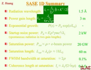
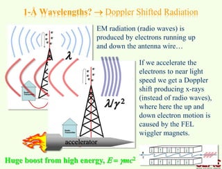
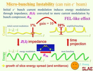
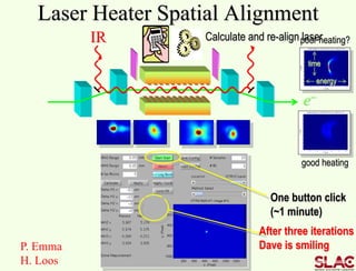
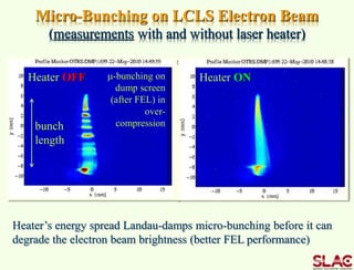
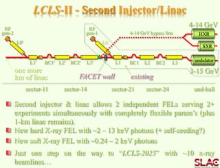
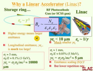
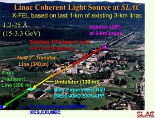
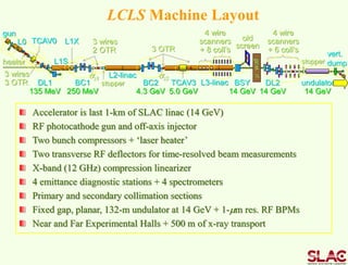
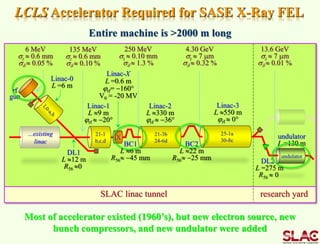
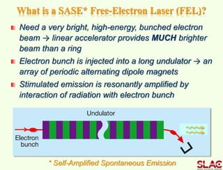
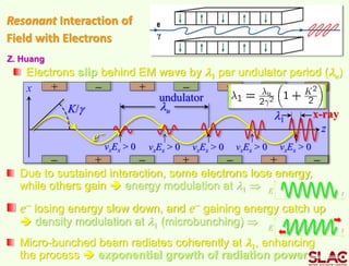
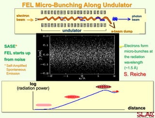
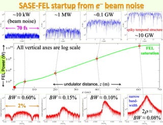
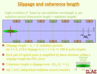
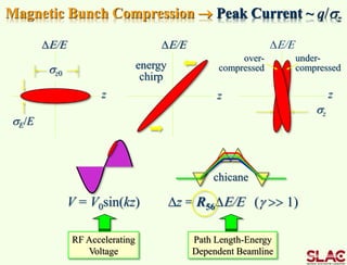
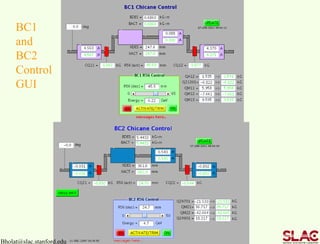
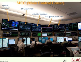
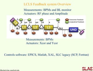
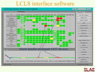
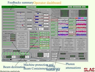
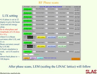
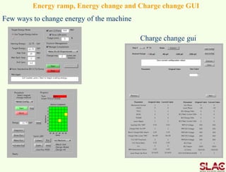
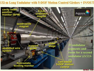
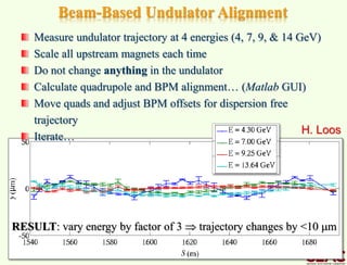
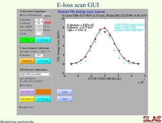
bholat@slac.stanford.edu
LCLS tuning
Hanif Bholat
June 29,2011
Bholat@slac.stanford.edu
Outline
• Scientific motivation for FEL (one example)
• Principal of FEL
• Important parameters of FEL
• Systematic tuning the FEL parameters
• User’s requirements
• Improvement and future plans
• Conclusion and Q&A.
Bholat@slac.stanford.edu
Protein before and after folding
Amyloidoses
Alzheimer�s disease
Prion diseases
Misfolding and cancer
Protein folding diseases
t = 0
Bholat@slac.stanford.edu
t = 25 fs
t = 50 fs
…which is being imaged with intense x-rays
BEFORE its destruction
Coulomb Explosion of Lysozyme (50 fs)
J. Hajdu, Uppsala
1-Å spatial
resolution
with hard
x-rays
femtosecond
short pulses to
resolve atomic and
molecular dynamics
Bholat@slac.stanford.edu
Experimental Hutches at Linac Coherent Light Source
•AMO: Atomic, Molecular & Optical Science
This instrument will enable the study of the interaction between the extremely intense
LCLS X-ray pulses and the basic constituents of matter: atoms and molecules.
• CXI: Coherent X-ray Imaging
This instrument will take advantage of the extremely bright, ultrashort LCLS pulses of
hard X-rays to allow imaging of non-periodic nanoscale objects, including single or
small clusters of biomolecules at or near atomic resolution.
• MEC: Matter in Extreme Conditions
This proposed instrument will observe matter at temperatures exceeding 10,000 Kelvin
and at pressures 10 million times the earth's atmospheric pressure at sea-level, enabling
unprecedented understanding of exotic states of matter.
•SXR: Soft X-ray Materials Science
This instrument will enable the high brightness and timing capability of the LCLS to be
applied to scattering and imaging experiments that require the use of soft X-rays.
•XCS: X-ray Correlation Spectroscopy
This instrument will observe dynamical changes of large groups of atoms in condensed
matter systems over a wide range of time scales.
• XPP: X-ray Pump Probe
This instrument will predominantly use a fast optical laser to generate transient states of
matter, and the hard X-ray pulse from the LCLS to probe the structural dynamics
initiated by the laser excitation.
•
Bholat@slac.stanford.edu
Experimental Hutches at Linac Coherent Light Source
Techniques Electron time-of-flight spectroscopy
Ion time-of-flight spectroscopy
Ion imaging
Ion momentum spectroscopy
X-ray scattering
Sample Environment A variety of pulsed and continuous gas, liquid and particle injectors
pulsed Proch-Trickl, Even-Lavie or Parker gas valves with heating and cooling options
single or double skimmer chambers for gas beams
motorized XYZ paddle for solid samples
liquid jet for biological samples
aerosol jet of particulate samples
Scientific Applications Coherent X-ray imaging on single sub-micron particles
Macromolecular Nanocrystallography
High Fluence X-ray interactions with matter
Time-resolved imaging and scattering with hard x-rays
Techniques and Scattering
Geometry
Forward scattering on target-mounted samples andfree-standing injected particles
Back-scattering
Ion Time-of-flight
Bholat@slac.stanford.edu
Scientific Application Time-resolved spectroscopy and scattering with ultrafast and ultraintense soft X-rays at the LCLS
Techniques X-ray Emission Spectroscopy (XES)
X-ray Photoelectron Spectroscopy (XPS)
X-ray Absorption Spectroscopy (XAS)
Coherent Imaging
Fourier Transform Holography
Diffraction
Sample Environment A wide range of experimental setups in UHV and HV conditions
Experimental Hutches at Linac Coherent Light Source
Scientific Applications X-ray PhotonCorrelation Spectroscopy (XPCS)
Coherent X-ray Scattering (CXS)
Scattering Geometries Small Angle X-ray Scattering (SAXS)
Grazing incidence Scattering (GI-SAXS,GID)
Wide Angle X-ray Scattering/Diffraction
Scientific Applications Femtosecond Structural Dynamics
X-ray Interactions with Matter
X-ray Techniques Wide Angle X-ray Scattering/Diffraction
Small Angle X-rays Scattering
X-ray Absorption Spectroscopy
X-ray Emission Spectroscopy
Bholat@slac.stanford.edu
LightSourcesat~0.1nm
1010
H.-D. Nuhn,
H. Winnick
storage
rings
Free-
Electron
Lasers
represent a huge
technical
advance with:
 1010 increase of peak
brightness,
 coherent x-rays,
 Femtosec pulses,
and
 Angstrom
wavelengths
LCLS I
LCLS II
Bholat@slac.stanford.edu
Why a Linac-Based Free-Electron Laser* ?
•“Recent” advances in high-brightness RF photocathode guns
•Longitudinal emittance from linac is ~103 smaller than ring
•Bunch length can be <100 fs and with small energy spread
•Experience from linear collider operation and study (SLC,
TESLA, JLC, NLC, CLIC)
•The last 1-km of the SLAC linac is available
•FEL produces unprecedented brightness and fsec pulses
Use SASE** (Self-Amplified Spontaneous Emission) 
no mirrors or seed-lasers at 1-Å wavelengths
* Motz 1950; Phillips 1960; Madey 1970
** Kondratenko, Saldin 1980; Bonifacio, Pellegrini 1984
Why a Linear Accelerator (Linac)?
ex ~ g 2
sz  5 mm,
sE/E  0.1% (1 GeV),
gez = szsE/mc2  10000
mm
Storage ring…
Higher energy means larger
emittance
Longitudinal emittance, gez ,
is much too large!
Much smaller gez
Emittance scaling (1/g )!
But lower repetition rate
ex ~ 1/ggez < 10 mm
RF Photocathode
Gun (or SCSS gun) Linac
zyx
e
e
N
B
eee
~
sz  1 mm,
sE/E  0.05% (5 MeV),
gez = szsE/mc2  5 mm
Linac Coherent Light Source at SLAC
Injector (35º)
at 2-km point
Existing 1/3 Linac (1 km)
(with modifications)
Near Experiment Hall
(NEH) AMO,SXR,XPP
Far Experiment Hall(FEH)
XCS,CXI,MEC
Undulator (130 m)
X-FEL based on last 1-km of existing 3-km linac
New e- Transfer
Line (340 m)
1.2-25 Å
(15-3.3 GeV)
X-ray
Transport
Line (200 m)
BC2
4.3 GeV
BSY
14 GeV
TCAV3
5.0 GeV
BC1
250 MeV
L1S
3 wires
2 OTR
L1X
4 wire
scanners
+ 8 coll’s
L2-linac
L3-linacDL1
135 MeV
L0
gun
TCAV0 old
screen3 OTR
sz1 sz2
3 wires
3 OTR stopper
heater
mwall
DL2
14 GeV
undulator
14 GeV
4 wire
scanners
+ 6 coll’s
vert.
dumpstopper
LCLS Machine Layout
Accelerator is last 1-km of SLAC linac (14 GeV)
RF photocathode gun and off-axis injector
Two bunch compressors + ‘laser heater’
Two transverse RF deflectors for time-resolved beam measurements
X-band (12 GHz) compression linearizer
4 emittance diagnostic stations + 4 spectrometers
Primary and secondary collimation sections
Fixed gap, planar, 132-m undulator at 14 GeV + 1-mm res. RF BPMs
Near and Far Experimental Halls + 500 m of x-ray transport
LCLS Accelerator Required for SASE X-Ray FEL
SLAC linac tunnel research yard
Linac-0
L =6 m
Linac-1
L 9 m
rf  -20°
Linac-2
L 330 m
rf  -36°
Linac-3
L 550 m
rf  0°
BC1
L 6 m
R56 -45 mm
BC2
L 22 m
R56 -25 mm DL2
L =275 m
R56  0
DL1
L 12 m
R56 0
undulator
L =130 m
6 MeV
sz  0.6 mm
s  0.05 %
135 MeV
sz  0.6 mm
s  0.10 %
250 MeV
sz  0.10 mm
s  1.3 %
4.30 GeV
sz  7 mm
s  0.32 %
13.6 GeV
sz  7 mm
s  0.01 %
Linac-X
L =0.6 m
rf= -160
V0 = -20 MV
rf
gun
21-3b
24-6d
X
25-1a
30-8c
...existing
linac
undulator
Most of accelerator existed (1960’s), but new electron source, new
bunch compressors, and new undulator were added
Entire machine is >2000 m long
21-1
b,c,d
Gun-Solenoid Assembly Cut-away view of gun (1.6 RF cells)
New Radio Frequency Photo-Cathode Gun
10 cmD. Dowell, E. Jongewaard
copper
cathode
Copper cathode (low QE, but stable)
UV laser illumination extracts electrons
Radio Frequency acc. fields (3 GHz)
Accelerate before space-charge blow up
Can produce very bright electron beam
3 GHz RF 120 MV/m
e-
UV
Injector Transverse Emittance <0.5 mm
135 MeV
0.25 nC
35 A
gex  0.43 mm
gey  0.46 mm
D. Dowell ,et al.
Exceptional beam
quality from S-
band Cu-cath. RF
gun…
Time-sliced emittance is even less: 0.4 mm
RF Photo-Cathode Gun & Spectrometer
e- (6 MeV)
e-
focusing
solenoid
RF gun
cathode (Cu)
UV Drive
Laser
spectrometer dipole
Q  0.25 nC
frep  120 Hz
Ecath  120 MV/m
fRF = 2856 MHz
gex,y  0.5 mm
Dt  3 ps
Real Gun-To-Linac Section
Need a very bright, high-energy, bunched electron
beam → linear accelerator provides MUCH brighter
beam than a ring
Electron bunch is injected into a long undulator → an
array of periodic alternating dipole magnets
Stimulated emission is resonantly amplified by
interaction of radiation with electron bunch
What is a SASE* Free-Electron Laser (FEL)?
* Self-Amplified Spontaneous Emission
X-rays
~100 m
z
x
Due to sustained interaction, some electrons lose energy,
while others gain  energy modulation at 1 
e- losing energy slow down, and e- gaining energy catch up
 density modulation at 1 (microbunching) 
Micro-bunched beam radiates coherently at 1, enhancing
the process  exponential growth of radiation power
u
e-
1
x-ray
Electrons slip behind EM wave by 1 per undulator period (u)
Z. Huang
+ - + - + -
- + - + - +
K/g
vxEx > 0
+
-
Resonant Interaction of
Field with Electrons
E t
E t
vxEx > 0 vxEx > 0vxEx > 0 vxEx > 0
undulator
FEL Micro-Bunching Along Undulator
SASE*
FEL starts up
from noise
* Self-Amplified
Spontaneous
Emission
log
(radiation power)
distance
electron
beam
undulator
photon
beam
e-beam dump
S. Reiche
Electrons form
micro-bunches at
the radiation
wavelength
(~1.5 Å)
~10 kW
(beam noise)
~1 MW ~0.1 GW
~10 GW
SASE-FEL startup from e- beam noise
BW ≈ 0.60% BW ≈ 0.15% BW ≈ 0.10%
2r ≈
BW ≈ 0.08%
spiky temporal structure
narrow
band-
width
All vertical axes are log scale
70 fs
2%
FEL
saturation
undulator distance, z (m)
FELPower(W)
+ - + - + -
- + - + - +
+
-
Slippage and coherence length
Light overtakes e- beam by one radiation wavelength 1 per
undulator period (interaction length = undulator length)
z
Slippage length = 1 × N undulator periods:
(at 1.5 Å, LCLS slippage is: ls ≈ 1.5 fs << 100-fs pulse length)
Each part of optical pulse is amplified by those electrons within a
slippage length (an FEL slice)
Coherence length is slippage over ~2LG (lc << ls)
ML ≈ Dz/lc independent radiation sources (modes)
N1
e-x-rays
slippage
length
Dz
~1 µm
Electron Beam Requirements for SASE FEL
eN < 1 µm at 1 Å, 15 GeV
<0.04% at Ipk = 3 kA,
K  3, u  3 cm, …
18LG ≈ 100 m for eN  1.5
µm
Need high peak current, low emittance, and small energy spread so that the x-ray
radiation power grows exponentially with undulator distance, z
P(z) = P0∙exp(z/LG)
FEL power reaches saturation at ~18LG
SASE performance depends exponentially on e- beam quality ! (challenge)
transverse emittance:
(volume occupied in phase space)
radiation wavelength (e.g., 1 Å)
relative energy spread:
peak current undulator period
beta function undulator ‘field’ = 0.93∙Bu
FEL gain length:
FEL parameter
sz0
DE/E
z
sz
under-
compressed
V = V0sin(kz)
RF Accelerating
Voltage
Dz = R56DE/E (g >> 1)
Path Length-Energy
Dependent Beamline
DE/E
z
sE/E
DE/E
z
energy
chirp
over-
compressed
chicane
Magnetic Bunch Compression  Peak Current ~ q/sz
Bholat@slac.stanford.edu
BC1
and
BC2
Control
GUI
Injector
summary LCLS summary
Undulator summary
FEL power in real time
Jitter summary
10/23/2016 26
MCC (Main Control Center)
Bholat@slac.stanford.edu
Controls software: EPICS, Matlab, XAL, SLC legacy (SCP, Fortran)
LCLS Feedback system Overview
Measurements: BPMs
Actuators: Xcor and Ycor
Measurements: BPMs and BL monitor
Actuators: RF phase and Amplitude
LCLS interface software
Alarm handler propagate OOT devices
Bholat@slac.stanford.edu
Operator dashboardFeedbacks summary
Machine protection and
Beam Containment summary
Tuning
Matlab gui
Beam destination
Photon
attenuations
Bholat@slac.stanford.edu
RF Phase scans
After phase scans, LEM (scaling the LINAC lattice) will follow
•L1S phase is set at 22
degree to give the beam
head and tail energy
chirp.
So at what phase and
Amplitude of L1X does
Cs=-Cx;
where Cs is Beam
curvature after L1S, and
Cx is
Beam curvature caused
by L1X RF.
LiTrack simulation is
used, set L1X need to
be
almost back phase to ~-
160 degree.
L1X setting
Bholat@slac.stanford.edu
Emittance measurement At different part of the LCLS machine
SLAC linac tunnel research yard
Linac-0
L =6 m
Linac-1
L 9 m
rf  -25°
Linac-2
L 330 m
rf  -41°
Linac-3
L 550 m
rf  0°
BC1
L 6 m
R56 -39 mm
BC2
L 22 m
R56 -25 mm DL2
L =275 m
R56  0
DL1
L 12 m
R56 0
undulator
L =130 m
6 MeV
sz  0.83 mm
s  0.05 %
135 MeV
sz  0.83 mm
s  0.10 %
250 MeV
sz  0.19 mm
s  1.6 %
4.30 GeV
sz  0.022 mm
s  0.71 %
13.6 GeV
sz  0.022 mm
s  0.01 %
Linac-X
L =0.6 m
rf= -160
21-1
b,c,d
...existing
linac
rf
gun
21-3b
24-6d
X
25-1a
30-8c
undulator
Bholat@slac.stanford.edu
Injector match guiSector 21 match guiSector 28 match guiLTU match gui
These match
Quads talk
heavily to
FEL power
Undulator match gui
Bholat@slac.stanford.edu
Correlation GUI
Most important tuning tool for the Operators!
Fast
control
PV
Control
PV
Read
PV list
Formula for Y axis
Bholat@slac.stanford.edu
Emittance tuning and Matching..
Match Quads
Emittance tuning
set points
Bholat@slac.stanford.edu
Emittance tuning and Matching..
Match Quads Emittance tuning Quads
Emittance tuning
set points
Bholat@slac.stanford.edu
Emittance tuning and Matching..
Li28 Match Quads
Emittance
tuning set
point for
Li28
Emittance tuning
set points for Li28
Bholat@slac.stanford.edu
Emittance tuning and Matching..
LTU Matching
Quads FEL tuning
knobs.
Emittance tuning
set points for LTU
Emittance tuning
set points
Bholat@slac.stanford.edu
Emittance tuning and Matching..
Undulator match
Quads FEL tuning
knobs.
e-
sz
sy
RF
‘streak’
V(t)
S-band (2856 MHz)
transverse RF deflector
off-axis
screen
single-shot, absolute
bunch length
measurement
e- Bunch Length Measured with Transverse RF Deflector
Deflector used to measure:
absolute bunch length,
time-sliced x-emittance,
time-sliced energy spread,
electron arrival time jitter
deflector OFF deflector ON
time
…one deflector at 135 MeV & another at 5 GeV
And slotted Foil Control gui
Bunch length GUI
Bunch length Measurement gui
P. Emma, M. Cornacchia, K.
Bane, Z. Huang, H. Schlarb
(DESY), G. Stupakov, D. Walz
Narrow or Double X-Ray Pulses from a Slotted Foil
PRL 92, 074801 (2004).
time (fs)
Power(GW)
0
10
5
0-150 fs
2 fs
0-6 mm
0.25 mm
pulses not
coherent
OTR screen in BC2
(30 cm up-beam of foil)
FELX-rayPulseEnergy(mJ)
Scan only the
single-slot section…
FEL power is proportional to slot width (short pulses?)
3-mm thick
moveable
Aluminum foil
Few ways to change energy of the machine
Energy ramp, Energy change and Charge change GUI
Charge change gui
132-m Long Undulator with 5-DOF Motion Control Girders + IN/OUT
33 undulator
segments and
room for a second
undulator (LCLS-
II)
cavity beam
position
monitor (BPM)
quadrupole
magnet
3.4-m
undulator
magnet
cam-based
5-DOF motion
control
slider
stage
hydrostatic
leveling monitor
support
girderstretched wire
system
Beam-Based Undulator Alignment
Measure undulator trajectory at 4 energies (4, 7, 9, & 14 GeV)
Scale all upstream magnets each time
Do not change anything in the undulator
Calculate quadrupole and BPM alignment… (Matlab GUI)
Move quads and adjust BPM offsets for dispersion free
trajectory
Iterate…
RESULT: vary energy by factor of 3  trajectory changes by <10 mm
H. Loos
Bholat@slac.stanford.edu
E-loss scan GUI
Also monitor
and calibrate
gas detector
readings
vary FEL power with oscillations & record e- energy loss
1.5 Å
FEL e- Energy-Loss Shows >2 mJ per X-ray Pulse
Horizontal
Dog-Leg
BPMs
Dumpline
BPMs
Vertical
Bend
10 MeV/e- (2.4 mJ)
 ~100 meters 
initial DEi
final DEf
DE = DEf - DEi
FELON
Electron Energy Loss & Spread Induced by FEL Gain
4.3 GeV, r = 15 Å, Ipk = 500 A
FEL OFFFEL ON
suppress FEL with oscillationallow FEL with straight orbit
FELOFF
0.05%
50MeV
Undulator, Dump-Line, and Screen
10 MeV
loss/e-
2.6 mJ @
830 eV
Bholat@slac.stanford.edu
Gain Length measurement GUI
Move horizontal correctors in front of each undulators.
Undulator Gain Length Measurement at 1.5 Å
gex,y = 0.4 mm (slice)
Ipk = 3.0 kA
sE/E = 0.01% (slice)
(25 of 33 undulators installed)
Lg = 3.3 m
Saturation length
of 60 m in 112-m
und.
<1 mm Undulator Quadrupole Remote Position Control
±4 mm
3-parameter fit
to 20 BPMs
along undulator
(y0, y0, and Dy)
Dy = 30 nrad kick due to quad
(y0, y0)
0.7 mm
backlash
<0.5 µm res.
Undulator Alignment Diagnostics (Stretched Wires & Hydraulic Levels)
Girder Numbers
6
-6
-4
-2
0
2
4
x[microns]
0 5 10 15 20 25 30 35
Calculated orbit change
Measured und. & quad moves
H.-D. Nuhn, THOA02
undulator
alignment drift
over 3 days
Undulator Taper Control Gui.
Bholat@slac.stanford.edu
Taper control
options, Set e- beam
parameter
Undulator Taper more than Doubles Power
1%
1.5 Å
5-mrad pole
cant angle
unmeasured range (>5 mm)
measured range (|x|  5 mm)
Wake (3 kA)  40 MeV
Spont. (13.6 GeV)  20 MeV
Post Sat. Taper  70 MeV
H.-D. Nuhn, THOA02
FEL Energy (YAG)
FEL-induced
Energy Loss (BPMs)
 ~100 meters 
4.6 MeV
Vary the FEL power and record e- energy loss
Total x-ray screen
signal vs. undulator
K-taper (yaw)
4.6 MeV at 0.25 nC
= 1.1 mJ or 0.8×10¹²
photons/pulse (15
GW at 75-fs FWHM
pulse length)
1.5 Å
Dumpline
BPMs
Undulator ‘Taper Scan’ Shows 1.1 mJ per X-ray Pulse
Dog-Leg
BPMs
FEL Intensity Jitter 9.6% rms at 1.5 Å over >1 hr
1.87 ± 0.18 mJ
30 Hz beam rate,
5 Hz sample rate,
10000 data
points,
SASE saturation
klystrontrips
> 1 hr
LCLS Parameter Changes
Machine Pulse Rate (1, 10, 30, 60, 120 Hz & one-shot)*
changed in seconds with one button push.
Wavelength (25 - 1.2 Å) changed in 5-60 minutes.
Pulse Energy (0 - 4 mJ) easily lowered, but may take 1-2 hrs
to achieve >2.5 mJ (depends on wavelength, etc).
Pulse Length (60 - 500 fs FWHM – for soft x-rays) easily
changed in 1 minute (closed loop control).
Peak FEL Power (0 - 40 GW) set by pulse length (increases
with peak current – see next slide).
Ultra-Short Pulse Length (<10 fs FWHM?) 20 pC - requires
1-2 hours to establish (starting from nominal 250-pC
conditions).
* Single shot and burst mode can be control by the users
Pulse Length Easily Adjusted (500-60 fs)*
X-Ray Pulse Energy
vs. Pulse Length
(2.5 – 3.8 mJ)
e- Peak
Current
vs. Pulse
Length
(500-4000 A)
Peak FEL
Power
vs. Pulse
Length
(5-40 GW)
e- bunch length is quickly adjustable (<1 min)
from 60 to 500 fs (hard x-rays: 60 to 100 fs)
1.7 keV, 250 pC, 23 of 33 undulators inserted
* for soft x-rays (0.5-2 keV)
Conclusions.
• Routine tuning can be and is done during beam
“delivery”. User’s consent usually required.
• Energy changes take away from “delivery” time.
Smaller energy changes are accomplished by
Energy ramp gui. Larger energy change require
multiple steps,
Load known good configuration close to desired
energy.
Activate Klystrons on the beam to match the
configuration energy.
LEM (scale LINAC lattice)
Run energy ramp gui to get to the desired energy.
Bholat@slac.stanford.edu
Conclusions.
Steer to “gold” orbit.
Standardize all the bend magnets
• Known problems:
Correctors don’t scale properly.
Muon Shield wall generate multipole
fields.
BX01/BX02 correctors.
50B1 degauss.
A4 BSY correctors remnant fields.
Bholat@slac.stanford.edu
Conclusions.
• One way to speed up large energy change
would be to establish every 500MeV “safe
zone” configuration file during Machine
Development (MD)
• Going to low charge ultra short pulse take
away time from delivery. There are many
steps involved, some are automated others
can’t be automated. (1-2hrs)
• There is an ongoing effort to create new tools
to configure LCLS machine efficiently and
repeatable manner so as to satisfy user
requirements.
Bholat@slac.stanford.edu
Acknowledgements
R.Akre, A.Brachmann,FJ. Decker, D. Dowell,
P.Emma, S. Giliveich, Z. Huang, S.Khan, H.
Loos, A.Novohatsky, HD. Nuhn, H.Smith,
M.Stanek, S. Tantawi, S. Weathersby, and
ALL THE OPERATORS.
Bholat@slac.stanford.edu
Thank you for your attention.
bholat@slac.stanford.edu
END
More slides
• FEL Summary
• LASER Heater
• LCLS II
Bholat@slac.stanford.edu
SASE 1D Summary
Radiation wavelength:
Power gain length:
Exponential growth: P(z) = P0 exp(z/LG)
Startup noise power: P0 ≈ Kr2gmc3/1
(spontaneous radiation in two gain lengths)
Saturation power: Psat ≈ r × e-beam power
Saturation length: Lsat ≈ u/r ≈ 18LG
FWHM bandwidth at saturation: ≈ 2r
Coherence length at saturation: lc ≈ 1/(2pr)
Z. Huang
3 m
2 kW
20 GW
60 m
0.1%
0.3 fs
1.5 Å
-
EM radiation (radio waves) is
produced by electrons running up
and down the antenna wire…
If we accelerate the
electrons to near light
speed we get a Doppler
shift producing x-rays
(instead of radio waves),
where here the up and
down electron motion is
caused by the FEL
wiggler magnets.
1-Å Wavelengths?  Doppler Shifted Radiation

accelerator
/g 2
Huge boost from high energy, E = gmc2
Micro-bunching Instability (can ruin e- beam)
Initial e- bunch current modulation induces energy modulation
through impedance, Z(), converted to more current modulation by
bunch compressor, R56


 growth of slice energy spread (and emittance)
time
projection
t
t
gain = 10
R56
Current
t
Energy
t
1% 10%initial current modulation
energy modulation more bunching
amplified bunching
Z. Huang
Z() impedance
FEL-like effect
Laser Heater Spatial Alignment
e-
IR Calculate and re-align laserpoor heating?
good heating
One button click
(~1 minute)
time
energy
After three iterations
Dave is smilingP. Emma
H. Loos
Micro-Bunching on LCLS Electron Beam
(measurements with and without laser heater)
Heater ONHeater OFF m-bunching on
dump screen
(after FEL) in
over-
compressionbunch
length
Heater’s energy spread Landau-damps micro-bunching before it can
degrade the electron beam brightness (better FEL performance)
undulator
X
L1 L2 L3BC1 BC2
LCLS-II - Second Injector/Linac
RF
gun-1
L0
3-15 GeV
sector-11 sector-21 sector-24sector-14
existing
und-hall
L3
HXR4-14 GeV bypass line
4-14 GeV
X
RF
gun-2
L1 L2BC1 BC2
L0
FACET wall
Second injector & linac allows 2 independent FELs serving 2+
experiments simultaneously with completely flexible param’s (plus
1-km linac remains).
New hard X-ray FEL with ~2 – 13 keV photons (+ self-seeding?)
SXR
New soft X-ray FEL with ~0.24 – 2 keV photons
Just one step on the way to “LCLS-2025” with ~10 x-ray
beamlines…
one more
km of linac

TUDORTMUND1

  • 1.
  • 2.
    Bholat@slac.stanford.edu Outline • Scientific motivationfor FEL (one example) • Principal of FEL • Important parameters of FEL • Systematic tuning the FEL parameters • User’s requirements • Improvement and future plans • Conclusion and Q&A.
  • 3.
    Bholat@slac.stanford.edu Protein before andafter folding Amyloidoses Alzheimer�s disease Prion diseases Misfolding and cancer Protein folding diseases
  • 4.
    t = 0 Bholat@slac.stanford.edu t= 25 fs t = 50 fs …which is being imaged with intense x-rays BEFORE its destruction Coulomb Explosion of Lysozyme (50 fs) J. Hajdu, Uppsala 1-Å spatial resolution with hard x-rays femtosecond short pulses to resolve atomic and molecular dynamics
  • 5.
    Bholat@slac.stanford.edu Experimental Hutches atLinac Coherent Light Source •AMO: Atomic, Molecular & Optical Science This instrument will enable the study of the interaction between the extremely intense LCLS X-ray pulses and the basic constituents of matter: atoms and molecules. • CXI: Coherent X-ray Imaging This instrument will take advantage of the extremely bright, ultrashort LCLS pulses of hard X-rays to allow imaging of non-periodic nanoscale objects, including single or small clusters of biomolecules at or near atomic resolution. • MEC: Matter in Extreme Conditions This proposed instrument will observe matter at temperatures exceeding 10,000 Kelvin and at pressures 10 million times the earth's atmospheric pressure at sea-level, enabling unprecedented understanding of exotic states of matter. •SXR: Soft X-ray Materials Science This instrument will enable the high brightness and timing capability of the LCLS to be applied to scattering and imaging experiments that require the use of soft X-rays. •XCS: X-ray Correlation Spectroscopy This instrument will observe dynamical changes of large groups of atoms in condensed matter systems over a wide range of time scales. • XPP: X-ray Pump Probe This instrument will predominantly use a fast optical laser to generate transient states of matter, and the hard X-ray pulse from the LCLS to probe the structural dynamics initiated by the laser excitation. •
  • 6.
    Bholat@slac.stanford.edu Experimental Hutches atLinac Coherent Light Source Techniques Electron time-of-flight spectroscopy Ion time-of-flight spectroscopy Ion imaging Ion momentum spectroscopy X-ray scattering Sample Environment A variety of pulsed and continuous gas, liquid and particle injectors pulsed Proch-Trickl, Even-Lavie or Parker gas valves with heating and cooling options single or double skimmer chambers for gas beams motorized XYZ paddle for solid samples liquid jet for biological samples aerosol jet of particulate samples Scientific Applications Coherent X-ray imaging on single sub-micron particles Macromolecular Nanocrystallography High Fluence X-ray interactions with matter Time-resolved imaging and scattering with hard x-rays Techniques and Scattering Geometry Forward scattering on target-mounted samples andfree-standing injected particles Back-scattering Ion Time-of-flight
  • 7.
    Bholat@slac.stanford.edu Scientific Application Time-resolvedspectroscopy and scattering with ultrafast and ultraintense soft X-rays at the LCLS Techniques X-ray Emission Spectroscopy (XES) X-ray Photoelectron Spectroscopy (XPS) X-ray Absorption Spectroscopy (XAS) Coherent Imaging Fourier Transform Holography Diffraction Sample Environment A wide range of experimental setups in UHV and HV conditions Experimental Hutches at Linac Coherent Light Source Scientific Applications X-ray PhotonCorrelation Spectroscopy (XPCS) Coherent X-ray Scattering (CXS) Scattering Geometries Small Angle X-ray Scattering (SAXS) Grazing incidence Scattering (GI-SAXS,GID) Wide Angle X-ray Scattering/Diffraction Scientific Applications Femtosecond Structural Dynamics X-ray Interactions with Matter X-ray Techniques Wide Angle X-ray Scattering/Diffraction Small Angle X-rays Scattering X-ray Absorption Spectroscopy X-ray Emission Spectroscopy
  • 8.
    Bholat@slac.stanford.edu LightSourcesat~0.1nm 1010 H.-D. Nuhn, H. Winnick storage rings Free- Electron Lasers representa huge technical advance with:  1010 increase of peak brightness,  coherent x-rays,  Femtosec pulses, and  Angstrom wavelengths LCLS I LCLS II
  • 9.
    Bholat@slac.stanford.edu Why a Linac-BasedFree-Electron Laser* ? •“Recent” advances in high-brightness RF photocathode guns •Longitudinal emittance from linac is ~103 smaller than ring •Bunch length can be <100 fs and with small energy spread •Experience from linear collider operation and study (SLC, TESLA, JLC, NLC, CLIC) •The last 1-km of the SLAC linac is available •FEL produces unprecedented brightness and fsec pulses Use SASE** (Self-Amplified Spontaneous Emission)  no mirrors or seed-lasers at 1-Å wavelengths * Motz 1950; Phillips 1960; Madey 1970 ** Kondratenko, Saldin 1980; Bonifacio, Pellegrini 1984
  • 10.
    Why a LinearAccelerator (Linac)? ex ~ g 2 sz  5 mm, sE/E  0.1% (1 GeV), gez = szsE/mc2  10000 mm Storage ring… Higher energy means larger emittance Longitudinal emittance, gez , is much too large! Much smaller gez Emittance scaling (1/g )! But lower repetition rate ex ~ 1/ggez < 10 mm RF Photocathode Gun (or SCSS gun) Linac zyx e e N B eee ~ sz  1 mm, sE/E  0.05% (5 MeV), gez = szsE/mc2  5 mm
  • 11.
    Linac Coherent LightSource at SLAC Injector (35º) at 2-km point Existing 1/3 Linac (1 km) (with modifications) Near Experiment Hall (NEH) AMO,SXR,XPP Far Experiment Hall(FEH) XCS,CXI,MEC Undulator (130 m) X-FEL based on last 1-km of existing 3-km linac New e- Transfer Line (340 m) 1.2-25 Å (15-3.3 GeV) X-ray Transport Line (200 m)
  • 12.
    BC2 4.3 GeV BSY 14 GeV TCAV3 5.0GeV BC1 250 MeV L1S 3 wires 2 OTR L1X 4 wire scanners + 8 coll’s L2-linac L3-linacDL1 135 MeV L0 gun TCAV0 old screen3 OTR sz1 sz2 3 wires 3 OTR stopper heater mwall DL2 14 GeV undulator 14 GeV 4 wire scanners + 6 coll’s vert. dumpstopper LCLS Machine Layout Accelerator is last 1-km of SLAC linac (14 GeV) RF photocathode gun and off-axis injector Two bunch compressors + ‘laser heater’ Two transverse RF deflectors for time-resolved beam measurements X-band (12 GHz) compression linearizer 4 emittance diagnostic stations + 4 spectrometers Primary and secondary collimation sections Fixed gap, planar, 132-m undulator at 14 GeV + 1-mm res. RF BPMs Near and Far Experimental Halls + 500 m of x-ray transport
  • 13.
    LCLS Accelerator Requiredfor SASE X-Ray FEL SLAC linac tunnel research yard Linac-0 L =6 m Linac-1 L 9 m rf  -20° Linac-2 L 330 m rf  -36° Linac-3 L 550 m rf  0° BC1 L 6 m R56 -45 mm BC2 L 22 m R56 -25 mm DL2 L =275 m R56  0 DL1 L 12 m R56 0 undulator L =130 m 6 MeV sz  0.6 mm s  0.05 % 135 MeV sz  0.6 mm s  0.10 % 250 MeV sz  0.10 mm s  1.3 % 4.30 GeV sz  7 mm s  0.32 % 13.6 GeV sz  7 mm s  0.01 % Linac-X L =0.6 m rf= -160 V0 = -20 MV rf gun 21-3b 24-6d X 25-1a 30-8c ...existing linac undulator Most of accelerator existed (1960’s), but new electron source, new bunch compressors, and new undulator were added Entire machine is >2000 m long 21-1 b,c,d
  • 14.
    Gun-Solenoid Assembly Cut-awayview of gun (1.6 RF cells) New Radio Frequency Photo-Cathode Gun 10 cmD. Dowell, E. Jongewaard copper cathode Copper cathode (low QE, but stable) UV laser illumination extracts electrons Radio Frequency acc. fields (3 GHz) Accelerate before space-charge blow up Can produce very bright electron beam 3 GHz RF 120 MV/m e- UV
  • 15.
    Injector Transverse Emittance<0.5 mm 135 MeV 0.25 nC 35 A gex  0.43 mm gey  0.46 mm D. Dowell ,et al. Exceptional beam quality from S- band Cu-cath. RF gun… Time-sliced emittance is even less: 0.4 mm
  • 16.
    RF Photo-Cathode Gun& Spectrometer e- (6 MeV) e- focusing solenoid RF gun cathode (Cu) UV Drive Laser spectrometer dipole Q  0.25 nC frep  120 Hz Ecath  120 MV/m fRF = 2856 MHz gex,y  0.5 mm Dt  3 ps
  • 17.
  • 18.
    Need a verybright, high-energy, bunched electron beam → linear accelerator provides MUCH brighter beam than a ring Electron bunch is injected into a long undulator → an array of periodic alternating dipole magnets Stimulated emission is resonantly amplified by interaction of radiation with electron bunch What is a SASE* Free-Electron Laser (FEL)? * Self-Amplified Spontaneous Emission X-rays ~100 m
  • 19.
    z x Due to sustainedinteraction, some electrons lose energy, while others gain  energy modulation at 1  e- losing energy slow down, and e- gaining energy catch up  density modulation at 1 (microbunching)  Micro-bunched beam radiates coherently at 1, enhancing the process  exponential growth of radiation power u e- 1 x-ray Electrons slip behind EM wave by 1 per undulator period (u) Z. Huang + - + - + - - + - + - + K/g vxEx > 0 + - Resonant Interaction of Field with Electrons E t E t vxEx > 0 vxEx > 0vxEx > 0 vxEx > 0 undulator
  • 20.
    FEL Micro-Bunching AlongUndulator SASE* FEL starts up from noise * Self-Amplified Spontaneous Emission log (radiation power) distance electron beam undulator photon beam e-beam dump S. Reiche Electrons form micro-bunches at the radiation wavelength (~1.5 Å)
  • 21.
    ~10 kW (beam noise) ~1MW ~0.1 GW ~10 GW SASE-FEL startup from e- beam noise BW ≈ 0.60% BW ≈ 0.15% BW ≈ 0.10% 2r ≈ BW ≈ 0.08% spiky temporal structure narrow band- width All vertical axes are log scale 70 fs 2% FEL saturation undulator distance, z (m) FELPower(W)
  • 22.
    + - +- + - - + - + - + + - Slippage and coherence length Light overtakes e- beam by one radiation wavelength 1 per undulator period (interaction length = undulator length) z Slippage length = 1 × N undulator periods: (at 1.5 Å, LCLS slippage is: ls ≈ 1.5 fs << 100-fs pulse length) Each part of optical pulse is amplified by those electrons within a slippage length (an FEL slice) Coherence length is slippage over ~2LG (lc << ls) ML ≈ Dz/lc independent radiation sources (modes) N1 e-x-rays slippage length Dz ~1 µm
  • 23.
    Electron Beam Requirementsfor SASE FEL eN < 1 µm at 1 Å, 15 GeV <0.04% at Ipk = 3 kA, K  3, u  3 cm, … 18LG ≈ 100 m for eN  1.5 µm Need high peak current, low emittance, and small energy spread so that the x-ray radiation power grows exponentially with undulator distance, z P(z) = P0∙exp(z/LG) FEL power reaches saturation at ~18LG SASE performance depends exponentially on e- beam quality ! (challenge) transverse emittance: (volume occupied in phase space) radiation wavelength (e.g., 1 Å) relative energy spread: peak current undulator period beta function undulator ‘field’ = 0.93∙Bu FEL gain length: FEL parameter
  • 24.
    sz0 DE/E z sz under- compressed V = V0sin(kz) RFAccelerating Voltage Dz = R56DE/E (g >> 1) Path Length-Energy Dependent Beamline DE/E z sE/E DE/E z energy chirp over- compressed chicane Magnetic Bunch Compression  Peak Current ~ q/sz
  • 25.
  • 26.
    Injector summary LCLS summary Undulatorsummary FEL power in real time Jitter summary 10/23/2016 26 MCC (Main Control Center)
  • 27.
    Bholat@slac.stanford.edu Controls software: EPICS,Matlab, XAL, SLC legacy (SCP, Fortran) LCLS Feedback system Overview Measurements: BPMs Actuators: Xcor and Ycor Measurements: BPMs and BL monitor Actuators: RF phase and Amplitude
  • 28.
    LCLS interface software LCLSinterface software Alarm handler propagate OOT devices
  • 29.
    Bholat@slac.stanford.edu Operator dashboardFeedbacks summary Machineprotection and Beam Containment summary Tuning Matlab gui Beam destination Photon attenuations
  • 30.
    Bholat@slac.stanford.edu RF Phase scans Afterphase scans, LEM (scaling the LINAC lattice) will follow •L1S phase is set at 22 degree to give the beam head and tail energy chirp. So at what phase and Amplitude of L1X does Cs=-Cx; where Cs is Beam curvature after L1S, and Cx is Beam curvature caused by L1X RF. LiTrack simulation is used, set L1X need to be almost back phase to ~- 160 degree. L1X setting
  • 31.
    Bholat@slac.stanford.edu Emittance measurement Atdifferent part of the LCLS machine
  • 32.
    SLAC linac tunnelresearch yard Linac-0 L =6 m Linac-1 L 9 m rf  -25° Linac-2 L 330 m rf  -41° Linac-3 L 550 m rf  0° BC1 L 6 m R56 -39 mm BC2 L 22 m R56 -25 mm DL2 L =275 m R56  0 DL1 L 12 m R56 0 undulator L =130 m 6 MeV sz  0.83 mm s  0.05 % 135 MeV sz  0.83 mm s  0.10 % 250 MeV sz  0.19 mm s  1.6 % 4.30 GeV sz  0.022 mm s  0.71 % 13.6 GeV sz  0.022 mm s  0.01 % Linac-X L =0.6 m rf= -160 21-1 b,c,d ...existing linac rf gun 21-3b 24-6d X 25-1a 30-8c undulator Bholat@slac.stanford.edu Injector match guiSector 21 match guiSector 28 match guiLTU match gui These match Quads talk heavily to FEL power Undulator match gui
  • 33.
    Bholat@slac.stanford.edu Correlation GUI Most importanttuning tool for the Operators! Fast control PV Control PV Read PV list Formula for Y axis
  • 34.
    Bholat@slac.stanford.edu Emittance tuning andMatching.. Match Quads Emittance tuning set points
  • 35.
    Bholat@slac.stanford.edu Emittance tuning andMatching.. Match Quads Emittance tuning Quads Emittance tuning set points
  • 36.
    Bholat@slac.stanford.edu Emittance tuning andMatching.. Li28 Match Quads Emittance tuning set point for Li28 Emittance tuning set points for Li28
  • 37.
    Bholat@slac.stanford.edu Emittance tuning andMatching.. LTU Matching Quads FEL tuning knobs. Emittance tuning set points for LTU Emittance tuning set points
  • 38.
    Bholat@slac.stanford.edu Emittance tuning andMatching.. Undulator match Quads FEL tuning knobs.
  • 39.
    e- sz sy RF ‘streak’ V(t) S-band (2856 MHz) transverseRF deflector off-axis screen single-shot, absolute bunch length measurement e- Bunch Length Measured with Transverse RF Deflector Deflector used to measure: absolute bunch length, time-sliced x-emittance, time-sliced energy spread, electron arrival time jitter deflector OFF deflector ON time …one deflector at 135 MeV & another at 5 GeV
  • 40.
    And slotted FoilControl gui Bunch length GUI Bunch length Measurement gui
  • 41.
    P. Emma, M.Cornacchia, K. Bane, Z. Huang, H. Schlarb (DESY), G. Stupakov, D. Walz Narrow or Double X-Ray Pulses from a Slotted Foil PRL 92, 074801 (2004). time (fs) Power(GW) 0 10 5 0-150 fs 2 fs 0-6 mm 0.25 mm pulses not coherent
  • 42.
    OTR screen inBC2 (30 cm up-beam of foil) FELX-rayPulseEnergy(mJ) Scan only the single-slot section… FEL power is proportional to slot width (short pulses?) 3-mm thick moveable Aluminum foil
  • 43.
    Few ways tochange energy of the machine Energy ramp, Energy change and Charge change GUI Charge change gui
  • 44.
    132-m Long Undulatorwith 5-DOF Motion Control Girders + IN/OUT 33 undulator segments and room for a second undulator (LCLS- II) cavity beam position monitor (BPM) quadrupole magnet 3.4-m undulator magnet cam-based 5-DOF motion control slider stage hydrostatic leveling monitor support girderstretched wire system
  • 45.
    Beam-Based Undulator Alignment Measureundulator trajectory at 4 energies (4, 7, 9, & 14 GeV) Scale all upstream magnets each time Do not change anything in the undulator Calculate quadrupole and BPM alignment… (Matlab GUI) Move quads and adjust BPM offsets for dispersion free trajectory Iterate… RESULT: vary energy by factor of 3  trajectory changes by <10 mm H. Loos
  • 46.
  • 47.
    Also monitor and calibrate gasdetector readings vary FEL power with oscillations & record e- energy loss 1.5 Å FEL e- Energy-Loss Shows >2 mJ per X-ray Pulse Horizontal Dog-Leg BPMs Dumpline BPMs Vertical Bend 10 MeV/e- (2.4 mJ)  ~100 meters  initial DEi final DEf DE = DEf - DEi
  • 48.
    FELON Electron Energy Loss& Spread Induced by FEL Gain 4.3 GeV, r = 15 Å, Ipk = 500 A FEL OFFFEL ON suppress FEL with oscillationallow FEL with straight orbit FELOFF 0.05% 50MeV Undulator, Dump-Line, and Screen 10 MeV loss/e- 2.6 mJ @ 830 eV
  • 49.
    Bholat@slac.stanford.edu Gain Length measurementGUI Move horizontal correctors in front of each undulators.
  • 50.
    Undulator Gain LengthMeasurement at 1.5 Å gex,y = 0.4 mm (slice) Ipk = 3.0 kA sE/E = 0.01% (slice) (25 of 33 undulators installed) Lg = 3.3 m Saturation length of 60 m in 112-m und.
  • 51.
    <1 mm UndulatorQuadrupole Remote Position Control ±4 mm 3-parameter fit to 20 BPMs along undulator (y0, y0, and Dy) Dy = 30 nrad kick due to quad (y0, y0) 0.7 mm backlash <0.5 µm res.
  • 52.
    Undulator Alignment Diagnostics(Stretched Wires & Hydraulic Levels) Girder Numbers 6 -6 -4 -2 0 2 4 x[microns] 0 5 10 15 20 25 30 35 Calculated orbit change Measured und. & quad moves H.-D. Nuhn, THOA02 undulator alignment drift over 3 days
  • 53.
    Undulator Taper ControlGui. Bholat@slac.stanford.edu Taper control options, Set e- beam parameter
  • 54.
    Undulator Taper morethan Doubles Power 1% 1.5 Å 5-mrad pole cant angle unmeasured range (>5 mm) measured range (|x|  5 mm) Wake (3 kA)  40 MeV Spont. (13.6 GeV)  20 MeV Post Sat. Taper  70 MeV H.-D. Nuhn, THOA02
  • 55.
    FEL Energy (YAG) FEL-induced EnergyLoss (BPMs)  ~100 meters  4.6 MeV Vary the FEL power and record e- energy loss Total x-ray screen signal vs. undulator K-taper (yaw) 4.6 MeV at 0.25 nC = 1.1 mJ or 0.8×10¹² photons/pulse (15 GW at 75-fs FWHM pulse length) 1.5 Å Dumpline BPMs Undulator ‘Taper Scan’ Shows 1.1 mJ per X-ray Pulse Dog-Leg BPMs
  • 56.
    FEL Intensity Jitter9.6% rms at 1.5 Å over >1 hr 1.87 ± 0.18 mJ 30 Hz beam rate, 5 Hz sample rate, 10000 data points, SASE saturation klystrontrips > 1 hr
  • 57.
    LCLS Parameter Changes MachinePulse Rate (1, 10, 30, 60, 120 Hz & one-shot)* changed in seconds with one button push. Wavelength (25 - 1.2 Å) changed in 5-60 minutes. Pulse Energy (0 - 4 mJ) easily lowered, but may take 1-2 hrs to achieve >2.5 mJ (depends on wavelength, etc). Pulse Length (60 - 500 fs FWHM – for soft x-rays) easily changed in 1 minute (closed loop control). Peak FEL Power (0 - 40 GW) set by pulse length (increases with peak current – see next slide). Ultra-Short Pulse Length (<10 fs FWHM?) 20 pC - requires 1-2 hours to establish (starting from nominal 250-pC conditions). * Single shot and burst mode can be control by the users
  • 58.
    Pulse Length EasilyAdjusted (500-60 fs)* X-Ray Pulse Energy vs. Pulse Length (2.5 – 3.8 mJ) e- Peak Current vs. Pulse Length (500-4000 A) Peak FEL Power vs. Pulse Length (5-40 GW) e- bunch length is quickly adjustable (<1 min) from 60 to 500 fs (hard x-rays: 60 to 100 fs) 1.7 keV, 250 pC, 23 of 33 undulators inserted * for soft x-rays (0.5-2 keV)
  • 59.
    Conclusions. • Routine tuningcan be and is done during beam “delivery”. User’s consent usually required. • Energy changes take away from “delivery” time. Smaller energy changes are accomplished by Energy ramp gui. Larger energy change require multiple steps, Load known good configuration close to desired energy. Activate Klystrons on the beam to match the configuration energy. LEM (scale LINAC lattice) Run energy ramp gui to get to the desired energy. Bholat@slac.stanford.edu
  • 60.
    Conclusions. Steer to “gold”orbit. Standardize all the bend magnets • Known problems: Correctors don’t scale properly. Muon Shield wall generate multipole fields. BX01/BX02 correctors. 50B1 degauss. A4 BSY correctors remnant fields. Bholat@slac.stanford.edu
  • 61.
    Conclusions. • One wayto speed up large energy change would be to establish every 500MeV “safe zone” configuration file during Machine Development (MD) • Going to low charge ultra short pulse take away time from delivery. There are many steps involved, some are automated others can’t be automated. (1-2hrs) • There is an ongoing effort to create new tools to configure LCLS machine efficiently and repeatable manner so as to satisfy user requirements. Bholat@slac.stanford.edu
  • 62.
    Acknowledgements R.Akre, A.Brachmann,FJ. Decker,D. Dowell, P.Emma, S. Giliveich, Z. Huang, S.Khan, H. Loos, A.Novohatsky, HD. Nuhn, H.Smith, M.Stanek, S. Tantawi, S. Weathersby, and ALL THE OPERATORS. Bholat@slac.stanford.edu
  • 63.
    Thank you foryour attention. bholat@slac.stanford.edu END
  • 64.
    More slides • FELSummary • LASER Heater • LCLS II Bholat@slac.stanford.edu
  • 65.
    SASE 1D Summary Radiationwavelength: Power gain length: Exponential growth: P(z) = P0 exp(z/LG) Startup noise power: P0 ≈ Kr2gmc3/1 (spontaneous radiation in two gain lengths) Saturation power: Psat ≈ r × e-beam power Saturation length: Lsat ≈ u/r ≈ 18LG FWHM bandwidth at saturation: ≈ 2r Coherence length at saturation: lc ≈ 1/(2pr) Z. Huang 3 m 2 kW 20 GW 60 m 0.1% 0.3 fs 1.5 Å -
  • 66.
    EM radiation (radiowaves) is produced by electrons running up and down the antenna wire… If we accelerate the electrons to near light speed we get a Doppler shift producing x-rays (instead of radio waves), where here the up and down electron motion is caused by the FEL wiggler magnets. 1-Å Wavelengths?  Doppler Shifted Radiation  accelerator /g 2 Huge boost from high energy, E = gmc2
  • 67.
    Micro-bunching Instability (canruin e- beam) Initial e- bunch current modulation induces energy modulation through impedance, Z(), converted to more current modulation by bunch compressor, R56    growth of slice energy spread (and emittance) time projection t t gain = 10 R56 Current t Energy t 1% 10%initial current modulation energy modulation more bunching amplified bunching Z. Huang Z() impedance FEL-like effect
  • 68.
    Laser Heater SpatialAlignment e- IR Calculate and re-align laserpoor heating? good heating One button click (~1 minute) time energy After three iterations Dave is smilingP. Emma H. Loos
  • 69.
    Micro-Bunching on LCLSElectron Beam (measurements with and without laser heater) Heater ONHeater OFF m-bunching on dump screen (after FEL) in over- compressionbunch length Heater’s energy spread Landau-damps micro-bunching before it can degrade the electron beam brightness (better FEL performance)
  • 70.
    undulator X L1 L2 L3BC1BC2 LCLS-II - Second Injector/Linac RF gun-1 L0 3-15 GeV sector-11 sector-21 sector-24sector-14 existing und-hall L3 HXR4-14 GeV bypass line 4-14 GeV X RF gun-2 L1 L2BC1 BC2 L0 FACET wall Second injector & linac allows 2 independent FELs serving 2+ experiments simultaneously with completely flexible param’s (plus 1-km linac remains). New hard X-ray FEL with ~2 – 13 keV photons (+ self-seeding?) SXR New soft X-ray FEL with ~0.24 – 2 keV photons Just one step on the way to “LCLS-2025” with ~10 x-ray beamlines… one more km of linac